 |
in VISTA Cluster Rendering System |
|
in VISTA Cluster Rendering System |
| 1. Alpha Adjustment |
| 2. Axis Rotation |
| 3. Subset Observing by Region Selection |
| 4. Range Selection |
| 5. Cluster Marking and Unmarking |
| 6. Automated Rendering |
| 7. Random Rendering |
| 8. Label Loading |
9.
Auxiliary Operations
|
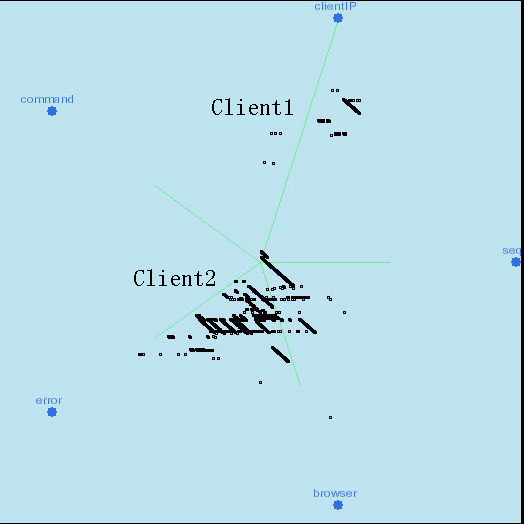
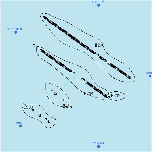
Alpha adjustment is used to change the projection plane. The alpha value is represented by the axis length( the scale of the absolute alpha value |alpha| ), and the axis color (green for positive values and yellow for negative values). Alpha adjustment increases or decreases the contribution of the particular attribute to the visualization. In the extended version, we also allow users to visualize the datasets that contain a few categorical data attributes. The categorical attributes are numerized by hashing the categorical values to the integers in range 0..n-1, where n is the number of all categories in the attribute. The numeric representation of categories is then normalized to [0, 1] like the other numeric attributes. When continuously adjusting the alpha value of a categorical attribute that has only a few categorical values, a user can see the point clouds that are identified by different categorical values moving in different directions and speeds. An example of web log dataset is shown in the Figure 1. The user can scale up the alpha value of the "ClientIP" attribute to check the distribution of the data points having different ClientIP. With the alpha adjustment only, we can see there are two groups in terms of the "ClientIP" attribute.
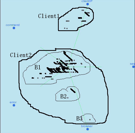
Alpha adjustment is also a natural way to expanding and collapsing clusters hierarchically. In Figure, after scaling up the "ClientIP" attribute, a subsequent scaling of "Browser" attribute shows that there are three sub-clusters (MSIE, Mozilla and Mozilla for NT) in the cluster "Client2", but there is no more sub-cluster in the cluster "Client1"(MSIE only).
The user uses the alpha widget to do alpha adjustment. After a dataset is loaded, the axes (i = 1, 2, ... , k), which correspond to the k dimensions, are created, and the initial alpha values are set to 0.5. To change alpha values, you need to set the operation mode to "change alpha". By pressing and holding the mouse button on alpha widget, the corresponding alpha value is increased, and by pressing mouse button plus "Ctrl" key the alpha value is decreased.
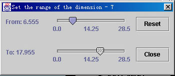
Figure 5a. The range selection of a numeric attribute
Axis rotation changes the direction of an axis. When several axes are rotated to the same direction, their contribution to the resultant visualization is aggregated. To contrast the effect of two sets of interesting attributes, the user can place the two sets of axes in two opposite directions and move aside other uninteresing attributes. For instance, in year-1984 house voting dataset we want to observe the tradeoff between votes to the education expense (the attribute: education-spending) and to the military/communication budgets (attributes: anti-satellite-test-ban and mx-missile). We rotate the axis (#13 education-spending) to the up-right corner and the other two (#8 anti-satellite-test-ban and #10 mx-missile) to the bottom-left corner. The visualization shows that most congressmen think that the military/communication budgets are much more important than the education expense.
Axis rotation can also be used to observe the relationship between any pair of attributes in a precise way. The user can rotate the target axes to two perpendicular directions and then set the a values of other attributes to 0, which becomes a standard 2D plot. For example, we want to observe the relationship between the attributes "Command" and "Error Code" in the web log dataset, where the user wants to find out the commands causing a certain error code, such as the error code "500".

VISTA system provides subset selection by free-drawing the region you want to observe in detail. To begin subset selection, firstly the user needs to shift the operation mode to "subset selection". To draw the boundary, put the mouse pointer to any beginning point on the boundary, then drag the mouse and enclose the boundary. The ending point does not need to be exactly at the beginning point. Subset selection will automatically enclose the area by connecting the ending point and the beginning point. Subset selection can also be done on the selected subset, which enables the user to observe the dataset hierarchically. Subset selection combined with zooming is especially useful when we need to explore a large amount of data points in a dense area. One example for the dataset DS1 shows how to hierarchically explore a dataset. DS1 has five clusters - one big spherical, two small spherical and two connected elliptical clusters. In the initial visualization (Figure 6a), we can see three clusters. The other two clusters may hide in the largest cluster. We select and zoom in the large cluster to see if there are other hidden clusters (Figure 6b). By using alpha parameter adjustment and zooming, together with subset selection, we can easily observe the detail of any part of the dense area. Figure 6c shows the detail of the select largest cluster in Figure 6b. In Figure 6c, we can see there are two overlapped clusters hidden in the large cluster. By adjusting the alpha values of different dimensions, we move the overlapped clusters out of the large cluster. Finally, zooming out and restoring the shaded data points, we find the five clusters in the visualization.
Range selection is another subset selection, which selects a subset by specifying a range of one attribute. In current version, we only implement range selection for single attribute. In the future version, the system can combine ranges of different attributes with some logical operations, such as AND or OR two selections. To activate the range selection, click right mouse button on an alpha widget. The range selection dialog box will appear at the top-right corner of the screen. Because we also allow to explore datasets that contains categorical data attributes, two kinds of range selection dialog boxes are provided for numerical and categorical data, respectively. The range selection dialog box for numerical data has two sliders, allowing users to selection the lower and upper bounds of the range. The range selection dialog box for categorical data has the list of all categorical values in this attribute. The user can choose one or multiple categories. When the user changes the numerical range or category selections, the corresponding selected data points are shown in red color. The user, then, can do all of the operations that work on subsets only. To recover the original unselected state, the user can re-open a range selection dialog box and press "Reset" button.
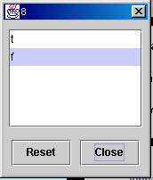
Figure 5b. Range selection of a categorical attribute
In order to mark a cluster, which will generate the definition of a cluster, you need to select the subset first, which can be done by region selection or range selection. After selecting the subset, click the button "Mark" to mark the cluster. To unmark a cluster, click mouse button on any point in the cluster when holding "Ctrl" key.
Automated rendering is mainly used in cluster rendering without any clue, which automatically increases or decreases the alpha value of the target attribute - the value is increased to 1 first and then decreased to -1, repeatedly. Automated rendering starts at the dimension 0 by default, however, the user can type in any valid dimension at the dimension box to change the beginning dimension. You can click the "Auto" button to start the rendering, or stop the rendering by the "Stop" button. You can also switch to the next/previous dimension by clicking "Next" or "Prev" button. Automated rendering provides a convenient way to adjust alpha values, when the number of dimensions is large.
Random rendering automatically changes all of the alpha values in a random amount at the same time. With random rendering for certain time, the user may find some interesting visualizations, which may not be easily found by step-by-step alpha adjustment.
Label loading can be used when cluster labels exist. The cluster label set is abstracted from the dataset that has already been labeled, or generated by other clustering systems. After loading the label set, the data points in different clusters are shown in different colors and different shapes. The user's task is to find the best boundaries that can separate all clusters well. The resultant visualization is saved as "cluster map" for ClusterMap labeling algorithm.
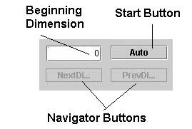
Figure 6. Controls for Automated Rendering