Project 1: Image Filtering and Hybrid Images
Image Filtering is a image processing technique useful for modifying images by applying various effects to it like blurring, sharpening etc. In addition to the spatial domain properties of an image, image filtering makes use of its properties in frequency domain as well. This allows effects like blurring, hybrid imaging etc. In this project, we implement Linear Image Filtering, and Hybrid Images. In Linear image filtering, a kernel matrix is used as a filter to modify the properties of the image. In spatial domain, the kernel (interchangeably called filter in this document) is used as a sliding window over the image. Each intensity of each pixel of the image is determined by convolution of the image with this sliding window kernel with the section of the image surrounding the target pixel. Hybrid Images are generated by superimposing two images that are filtered such that they contain different frequencies. This makes the viewed perceive both different images depending on his or her distance from the image, and size of the image. The two filtered images are created by using linear image filtering. The method used in this project for these two image processing techniques is described in detail in the following sections.
Image Filtering
Image Filtering uses convolution in spatial domain to apply a matrix with specific properties to an input image. In this project, we apply the filter as a sliding window over the image. The intensity of each pixel in the output image is calculated by element-wise multiplication and summation of filter with a block of the image surrounding the target pixel. This can be visualised as shown in Figure 1.

Figure 1: Example of linear filtering in spatial domain.
In figure 1, we see the input image f(x,y), and the filter h(x,y). The output is g(x,y) which is generated using equation 1 given below.

Equation 1: Output image's (g) pixel value is determined as a weighted sum of input image's (f) and filter's (h) pixel values.
In figure 1, we see the highlighted output pixel g(2,2) is calculated by element wise multiplication and sum of highlighted sub-matrix of input image f and filter h. In out project, we support only filters with odd height and width. We have implemented my_imfilter.m which does the filtering. The input parameters to this function are the input image and the filter. my_imfilter.m supports both greyscale and RGB images. For greyscale image, we element-wise mupltiply the filter with the image using two for loops. The outer for loop traverses along the height of the image, while the inner for loop traverses along the width. For the RGB image, we use repmat() function of matlab to create a 3D replica of the filter, and then element-wise multiply with the RGB image. This saves us from using three nested for loops, which would take higher computational time.
% loop over, and .multiply
% colour_im is the number of dimensions in the image.
% A 2 dimension image matrix is greyscale.
% A 3 dimensions image matrix is RGB.
% row_filter is height of filter.
% col_filter is width of filter.

if (colour_im == 2)
 for r = 1:size(image_pad,1) - row_filter + 1
  for c = 1:size(image_pad,2) - col_filter + 1
   filtered_image(r,c) =  sum(sum(image_pad(r : r+row_filter-1, c:c+col_filter-1) .* filter));
  end
 end
elseif (colour_im > 2)
 filter3D = repmat(filter, [1,1,3]);
 for r = 1:size(image_pad,1) - row_filter + 1
  for c = 1:size(image_pad,2) - col_filter + 1
   if min(size(filter)) == 1
    filtered_image(r,c,:) =  sum(image_pad(r : r+row_filter-1, c:c+col_filter-1,:) .* filter3D(:,:,:));
   else
    filtered_image(r,c,:) =  sum(sum(image_pad(r : r+row_filter-1, c:c+col_filter-1,:) .* filter3D(:,:,:)));
   end
  end
 end
end
We use the number of dimensions in the image to decide if it is a greyscale image or RGB image. To account for the corner pixels, we pad the input image such that the corner pixels are also center pixels when convolved with the filter. Thus, we pad ((filter_width - 1)/2) along the two sides of input image, and ((filter_height - 1)/2) along the top and bottom edges of input images. We use matlab's padarray() function for padding. We have used reflective padding for this project. Image filtering is performed using a number of filters viz., Identity filter, Box Filter (Small blur and large blur), Sobel filter, Laplacian high pass filter and an alternative to high pass filter i.e. original image - low pass filtered image. The result of applying these filters to figure 2(a) is shows in figure 2(b) to 2(g).
Results of Linear Image Filtering in table

Figure 2(a): Original Image. 
Figure 2(b): Image filtered with Identity Filter. 
Figure 2(c): Image filtered with Small blur box Filter. 
Figure 2(d): Image filtered with Large blur box Filter. 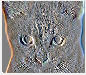
Figure 2(e): Image filtered with Sobel Filter. 
Figure 2(f): Image filtered with Discrete Laplacian High Pass Filter. 
Figure 2(g): Image filtered with alternative for High Pass filter. |
Hybrid Image
Hybrid Images are those which can be perceived as one image when viewed up-close, and a different image when viewed from a distance. This is achieved by playing around with the frequencies contained in the images. As we know, edges in an image in spatial domain translates as high frequencies in frequency domain. On the other hand, low frequencies translates as blurring in spatial domain. Thus, we use low pass and high pass filtering on two different, but well aligned images, and superimpose them. The high frequencies can be seen clearly when the viewer is looking closely, and these disappear, when looked at from a distance. Thus, the low frequencies of the other image takes form. The filter used for low pass is a gaussian filter. To obtain the high frequencies in the image, we simply subtract these low frequencies from the original image. Let us see generation of hybrid images using an example shows below in figure 2.


|
Figure 2(a): Original image einstein.bmp. Figure 2(b): Original image marilyn.bmp.


|
Figure 3(a): High frequency elements of einstein.bmp (cutoff freq 3).
Figure 3(b): Low frequency elements of marilyn.bmp (cutoff freq 4).

Figure 4: Hybrid image by superimposing Figure 3(a) and 3(b).
The amount of blurring of low frequency image depends on the deviation of the gaussian filter used. We generate the filter using fspecial() function of matlab which allows us to specify the size of the filter, and it's deviation. This deviation can be considered the cut-of frequency. Higher the cut off frequency of low pass filter, more is the blurring. This is because during convolution, larger number of pixels in input image surrounding a target pixel determine the value of the target pixel of output image. In this project we use two different cut-off frequencies for the high pass, and low pass filters. This allows us to closely modify the amount of low frequencies and high frequencies we wish to see in our final hybrid image to make it aesthetically appealing. Most of it is just manual tuning to obtain an image that can be perceived as both the constituting images at different distance. It must be noted that in addition to distance from viewer, the size of them image also result as different perceptions. Larger the image size, the view will have to view it from a further distance to be able to 'see' the hidden image. On the other hand, as we can see in figure 4, the smaller image starts to look like Marilyn even though we are viewing from the same distance.
Results of Hybrid Images in a table


Fig 5a: Original Images of dog and cat. |

Fig 5b: Hybrid Image of dog (cutoff freq 4) & cat (cutoff freq 9). |
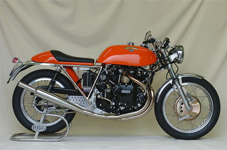

Fig 6a: Original Images of Motocycle and Bicycle. |

Fig 6b: Hybrid Image of motorbike (cutoff freq 5) and bicycle (cutoff freq 3). |


Fig 7a: Original Images of Submarine and Fish. |

Fig 7b: Hybrid Image of Submarine (cutoff freq 4) and Fish (cutoff freq 5). |


Fig 8a: Original Images of Bird and Plane. |

Fig 8b: Hybrid Image of Bird (cutoff freq 3) and Plane (cutoff freq 6). |
We can try generating hybrid images using our own images. For example in the figures shown below, we have tried to superimpose the image of a ballet dancer and a traffic police. We have also clicked images of a closed closet, and open closet and superimposed them. The original images, intermediate images, and resultant hybrid images are shown below.


|

|
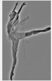
Figure 9a: Original Images of Police man and Ballet Dancer.
Figure 9b: Filtered Images of Police man (cutoff freq 4) and Ballet Dancer (cutoff freq 5).

Figure 9c: Hybrid Image.


|


|
Figure 10a: Original Images of Closed closet and Open Closet.
Figure 10b: Filtered Images of Closed closet (cutoff freq 4) and Open Closet (cutoff freq 5).

Figure 10c: Hybrid Image.
The major roadblock faced for creating new Hybrid images was alignment of original images. As we can see in the police man - ballet dance hybrid image in Fig 9c, the arms of both individuals are not well aligned, thus even from a distance, this can be seen. On the other hand, the closet is perfectly aligned in both images. Thus we see no issues with hybrid image.
The other observation that may disrupt the image is that most of the colour tends to be concentrated in low frequencies. As a result, the image containing high frequencies loses colour information. This can be clearly seen in Fig 8c. Although the original image of plane had a blue sky in the background, that is completely lost in the hybrid image. Similarly, in the closet image, the colour of the contents of closet are barely visible.