Project 1: Image Filtering and Hybrid Images
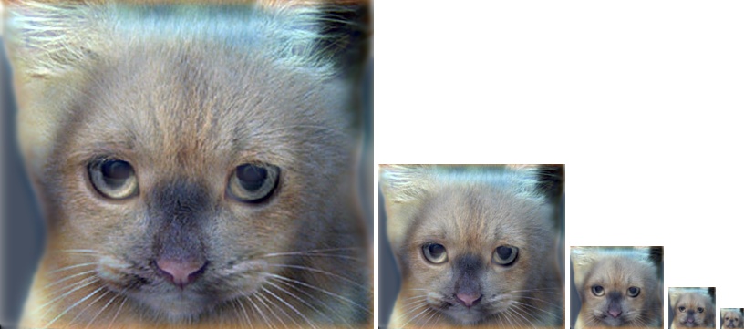
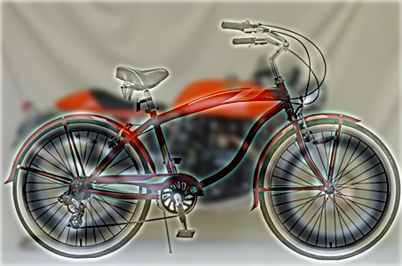
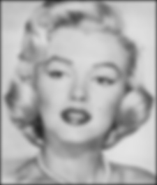
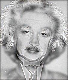
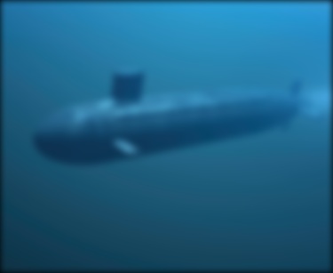
Example of a Hybrid Image.
This project involves the creation of an image filtering function, my_imfilter(), which imitates the default behavior of the built-in function imfilter() in MATLAB. The inputs to the my_imfilter() function are 1) The input image (color or grayscale is acceptable) and 2) The filter. The function supports filters of any size, as long as both dimensions are odd. If any dimension is even, the function throws an error. The function outputs a filtered image with the same resolution as the input image.
- Check size of filter - Throw error if any dimension is even, else proceed
- Boundary handling - Pad the input image with zeros. Pad size = (Filter - 1) / 2
- Check if image is in color or grayscale.
- If the image is in grayscale, separate image into chunks equal to the size of filter, perform dot product with the filter and add the values obtained. Here, a stride of 1 is used.
- If image is in color, separate it into R,G and B color channels and perform the above operation for all 3 color channels
- Recombine the filtered color channels to form an RGB image
- The function outputs the filtered image
The filter used is a Gaussian filter, of size cutoff_frequency*4+1 and standard deviation (in pixels) of cutoff_frequency. The centre element has the largest value, and the values of the other elements decrease symmetrically as distance from the centre increases. Cutoff_frequency is a free parameter and can be tuned for each image pair. For example, in the cat-dog pair, a cutoff_frequency of 7 works best.
Generating the Hybrid Image
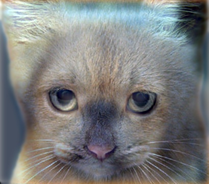
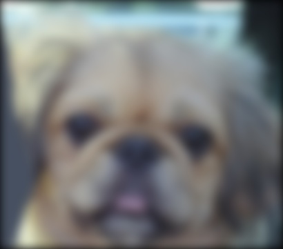
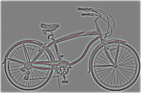
- Low Frequency Images - Gaussian blur is achieved by convolving the Gaussian filter with the image. This results in the blurring of the images, as the high frequencies are removed - low_frequency = my_imfilter(image, filter). The amount of blur depends on the cut off frequency value used.
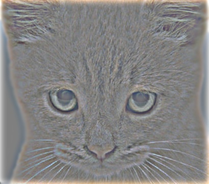
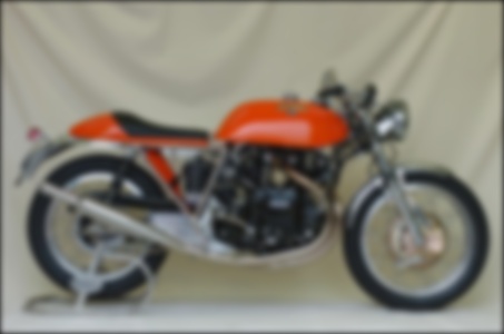
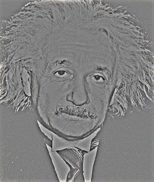
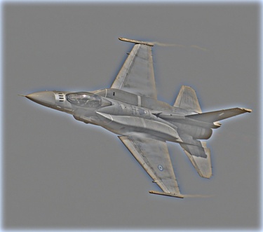
- High Frequency Images - High frequency images are generated by removing the low frequencies. This is done by subtracting the low frequency image from the original image, i.e., high_frequency = image - low_frequency.
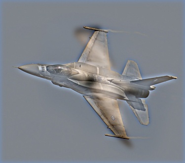
- Hybrid Images - Hybrid images are simply the sum of the high and low frequency images, i.e., hybrid = high_frequency + low_frequency.
Filtering:
The image filtering is performed as follows:
%Filtering code

result = zeros(size(image));

%Padding image
padx = floor(fwidth/2);
pady = floor(fheight/2);

image_new = padarray(image, [padx pady]);

if size(image, 3) == 3
    imagered = image_new(:,:,1);
    imagegreen = image_new(:,:,2);
    imageblue = image_new(:,:,3);
    for i = 1:imw
        for j = 1:imh
            tempr = imagered(i:i+(fwidth-1), j:j+(fheight-1)) .* filter;
            rr(i,j) = sum(tempr(:));
            tempg = imagegreen(i:i+(fwidth-1), j:j+(fheight-1)) .* filter;
            rg(i,j) = sum(tempg(:));
            tempb = imageblue(i:(i+fwidth-1), j:(j+fheight-1)) .* filter;
            rb(i,j) = sum(tempb(:));
        end
    end
    result = cat(3, rr, rg, rb);
else
    temp = image_new(i:i+(fwidth-1), j:j+(fheight-1)) .* filter;
    result(i,j) = sum(temp(:));
end

output = result;
Results in a table
|
|
|
|
|
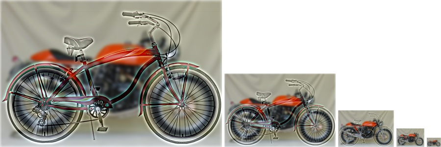
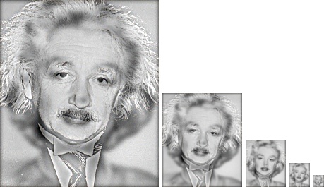
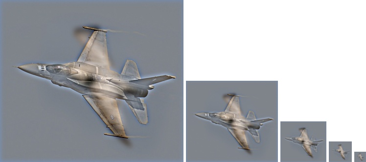
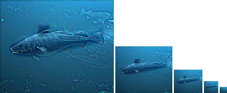
The first column shows all the images which have been blurred by removing the high frequencies. The second column displays images from which low frequencies have been removed. The third column of images are the hybrid images, the result of combining the low frequency and high frequency images. We observe that at close range, lor low values of scaling, high frequencies are most observable. However, as viewing distance increases, or the scaling increases, the blurred or low frequency image is perceived.