Project 1: Image Filtering and Hybrid Images
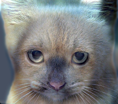
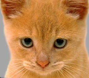
Example of a hybrid image of a pug and a tabby.
Hybrid images are composed of two images, where each have a range of frequencies filtered out. Two common examples are low-pass and high-pass filters. A low-pass filter removes high-frequency values from each color channel. Similarly, a high-pass filter removes low-frequency values. A common implementation of a low-pass filter uses a one-dimensional Gaussian to create a blur effect. Gaussian filters take a free parameter, the cutoff frequency, which specifies how exponential the filter fades to zero. A higher or lower cutoff frequency of the Gaussian may be specified to create a stronger or weaker blur, respectively. For the example images on this page, the cutoff was 5 +/-2.
The basic process of forming a hybrid image is as follows:
- Select two
MxNimages,image1andimage2. - Create a Gaussian filter.
- Filter
image1using the Gaussian to create a low-pass filtered version. - Create a high-pass of
image2. To do this simply,- Create a low-pass of
image2using the same Gaussian as above. - Element-wise subtract this low-pass from the original
image2.
- Create a low-pass of
- Combine the low-pass and high-pass images using element-wise addition into a final
MxNimage.
This process allows for images to be produced with two distinct properties: the low-pass image will be fairly distinct when viewed closely and the high-pass image is more visible from a distance.
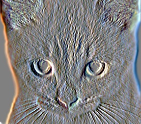
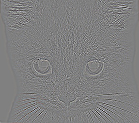
Images


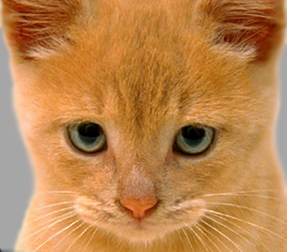
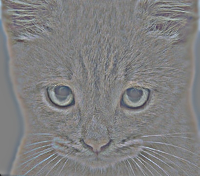
Above are the filtered images which went into the previous example hybrid. The dog had a low-pass filter applied to it and the cat was high-pass filtered. Hover over them to see the filters removed.
Example psuedocode of filtering algorithm
The code below provides a general overview of how the a 2D filter function works. For images with multiple color channels (RGB, RGBA, RGBD), each channel may be filtered separately.
% filtering
function filter ( image (MxN), mask (LxK) )
	new_image <- matrix of dimensions MxN
	foreach ( m,n in image dimensions )
		neighborhood <- KxL matrix surrounding image[m,n]
		new_image[m,n] <- sum(dot(mask, neighborhood)) % the dot product summed to a single value
	end
	return new_image
end
My implementation of filter made use of MATLAB's built-in dot function, which will perform the necessary matrix operation, saving the need for a third loop.
As opposed to filtering each color channel independently, which would require additional loops, I reproduced the filter matrix into the same number of channels as the image parameter.
MATLAB's dot function handles the dot product along the multiple dimensions.
The resulting product is then summed along the second dimension to produce a column of color values, therefore removing the need for a fourth loop.
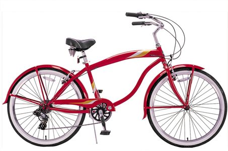
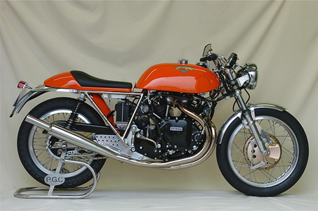
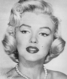
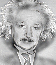
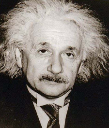
Examples of different images and filters

|
|
|
|
|
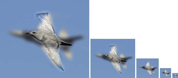
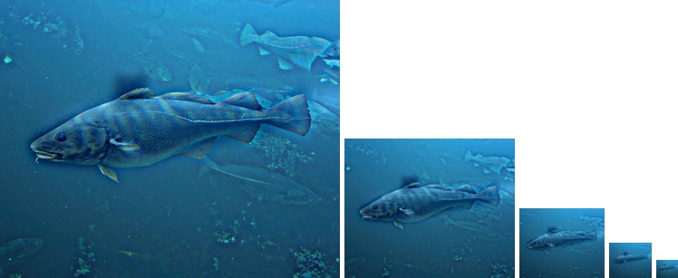
The illusion of distance may be simulated by progressivly scaling the images down, as shown in the last two rows of examples. Each downsampled image is a 0.5 scale of the previous. Another option is to look at the images through squinted eyes for more distance or through a pinhole for less. When creating a hybrid images, many factors may be considered. Firstly, images with more bright/light colors tend to be best for a low-pass. Likewise, dark colored images were usually high-passed. Secondly, the cutoff frequency for the Gaussian blur varies between image pairs, and is largely up to preference. The third row of examples shows different filters in action. The first image had an identity filter applied, which produces an image matching the input. The second image uses a Sobel filter, which focuses on highlighting edges in an image. In this case, it responds to horizontal gradients. The final image uses a Laplacian filter, an alternative to a high-pass filter where element-wise subtraction isn't necessary, however the result is not identical. In the end, trial and error of free parameters and image order lead to the best results, with the several examples shown above.