Project 1: Image Filtering and Hybrid Images
Image Filtering
The first part of this project dealt with creating an implementation of imfilter. In order to do this my goal was to apply a given filter to an image. The way we apply a filter to an image is by taking the dot product of the filter and image for every point in the image. We center the filter at a point of interest, multiply all image values with all corresponding filter values, and then put this result as the new value at that point in our output image. For colored images we have three layers in our original image, thus, we must apply our filter in this manner to all layers in our image. There is however one other consideration we must make when writing our algorithm. First, we must realize that for any filter larger than 1x1, when we center our filter on points near the edge of our image, our filter will overflow out of the image. To handle this scenario, I decided to pad my image with black pixels on the top and bottom by the floor of filter.height / 2 and on the left and right by the floor of filter.width / 2. Since we have the specification that our filter has odd valued dimensions, by adding padding of these sizes we ensure that even when our filter is applied to points on the corners of our image it does not overflow. Below shows the implementation of this padding:
imageDim = size(image);
filterDim = size(filter);
paddedImage = [];

% iterate through each layer of our image (the different colors if its colored)
for color = 1:imageDim(3)
    topBotPadSize = fix(filterDim(1) / 2);
    leftRightPadSize = fix(filterDim(2) / 2);
    % add a layer to our padded image which is our initial image with the specified padding
    paddedImage(:,:,color) = padarray(image(:,:,color), [topBotPadSize, leftRightPadSize]);
end
When it comes to the actual implementation of my filtering, I looped through the dimensions of my original image and applied the filter to the corresponding points on my padded image. I copied the result of the filter dotted with a portion of the padded image to a new image, which had the same dimensions as my original image. Below is the code performing this functionality:
% the array to store our filtered points
filteredArray = zeros(imageDim);
count = 0;
for z = 1:imageDim(3)
    for x = 1:imageDim(2)
        for y = 1:imageDim(1)
            imageLayer = paddedImage(:,:,z);
            % grab a filter-sized portion of the image centered based on
            % our original image dimensions
            extractedPixels = imageLayer(y:y+filterDim(1)-1, x:x+filterDim(2)-1);
            total = 0;
            % compute the dot product of the filter and these extracted
            % pixels
            for fx = 1:filterDim(2)
                for fy = 1:filterDim(1)
                    total = total + filter(fy, fx) * extractedPixels(fy, fx);
                end
            end
            % add the pixel to our filteredArray
            filteredArray(y, x, z) = total;
            count = count + 1;
        end
    end
end
output = filteredArray
We can break down the algorithm into the following steps:
- Pad our image based on the size of our filter.
- Compute the dot product of our filter with our padded image for each pixel in our original image (center the filter based on points in our original image).
- Add the result for each point to an output image of the same dimensions as our original image.
Examining Results:
Original Image
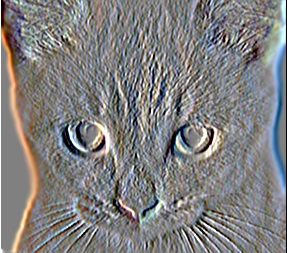
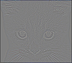
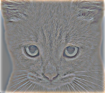
We examine the results of applying 6 different filters to our original image. We can tell very clearly that our image was padded with black pixels by observing the border of the picture in the Large Blur filter. The large blur takes adjacent pixels heavily into account, allowing us to see how our padding influenced the edges of the image. The large blur also takes many more pixels into account than the small blur, which uses a simple 3x3 filter to blur the image using only immediately adjacent pixels. However, by looking closely at the edges we can even see the padding creep into the image with our small blur. We also notice that, as expected, our identity filter returns an exact copy of our image. This is a good sanity check for our filtering algorithm. We also see that our Sobel Filter creates an image emphasizing edges, as is intended and expected. our sobel filter is a 3x3 filter which responds to horizontal gradients. We see this effect most prominent in the outline of our cat, which the sobel filter very clearly identifies on both sides of our image. When looking at our two high pass images we notice what we would expect. Both of our filters capture edges. In general a high pass filter will make an image appear sharper. We notice this perhaps most obviously with the cat's whiskers.
Identity Filter |
Small Blur (Box Filter) |
Large Blur (Gaussian Filter) |
Oriented Filter (Sobel) |
High Pass Filter (Discrete Laplacian) |
High Pass "filter" Alternative |
Hybrid Images
In terms of the hybrid image portion of this project I created a low-pass filtered version of one image and a high-pass filtered version of a second image. In order to create a low-pass filtered version I applied a filter to perform a Gaussian blur on an image. For the high-pass version I subtracted the initial image from the low-pass version of the same image in order to keep only the high frequencies. For each image I edited the cutoff_frequency parameter to find the best parameter for each image pair I combined. I then added together the two images to create the hybrid image. Below is the code that performs these operations:
cutoff_frequency = 7;
filter = fspecial('Gaussian', cutoff_frequency*4+1, cutoff_frequency);

low_frequencies = my_imfilter(image1, filter);
high_frequencies = image2 - my_imfilter(image2, filter);

hybrid_image = low_frequencies + high_frequencies;
Examining Results:
Let's begin by looking at a low pass and high pass version of two images we wish to create a hybrid image for:
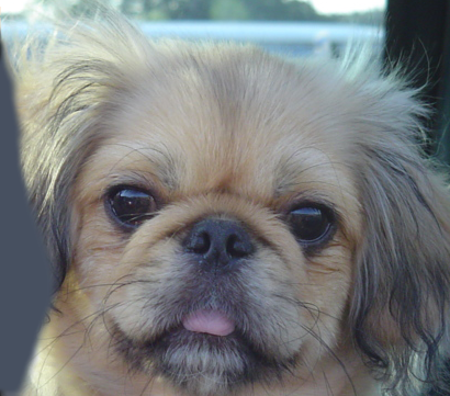
Original Dog |

Low Frequencies Dog |
|
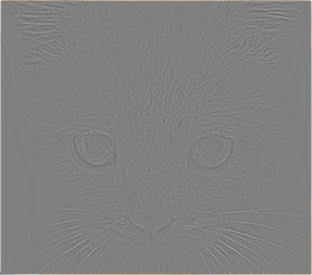
Original Cat |
High Frequencies Cat |
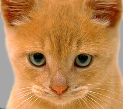
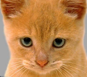
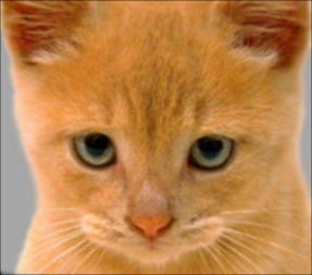
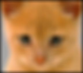
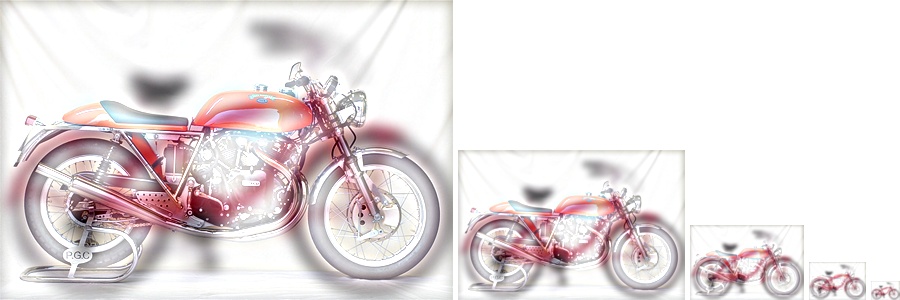
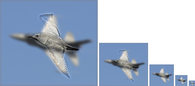
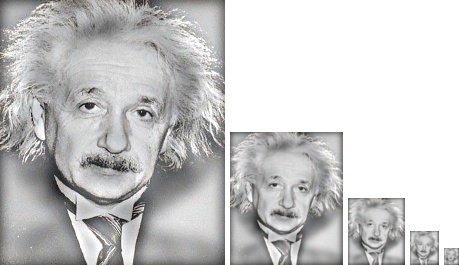
What happens when we add these two modified images together to create a hybrid image?
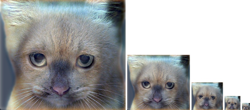
As you can see, the larger image looks more like a cat, whereas the smaller images each look more and more like a dog!
Let's take a look at some more images in their process to become hybrid images and the resulting hybrid images! Unless otherwise mentioned, I used a cutoff_frequency of 7, after trying various frequencies and looking for the one that provided the best distinction between the images when looking at the larger and smaller versions of the image. One interesting thing I noticed when editting cutoff_frequency was how it effected the images. For example, a higher cutoff frequency resulted in a blurrier low pass image whereas a lower cutoff make the low pass image sharper. This means that if we are having issues with the smaller images showing our low pass image clearly then we may want to use a higher cutoff frequency as this would result in a blurrier low pass image!
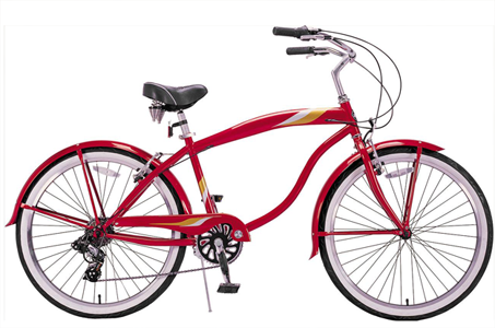
Original Bike |
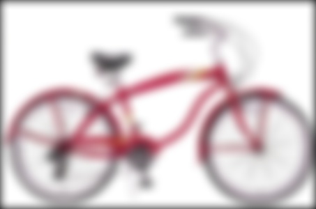
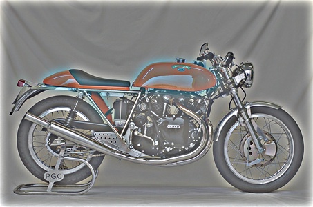
Low Frequencies Bike |
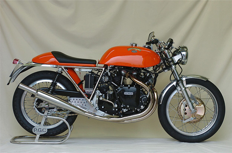
Original Motorcycle |
High Frequencies Motorcycle |
For the following image I changed my cutoff_frequency to 5, as I found that this maintained an obvious and sharp bird in the larger image while making the plane more prominent in the smaller images.
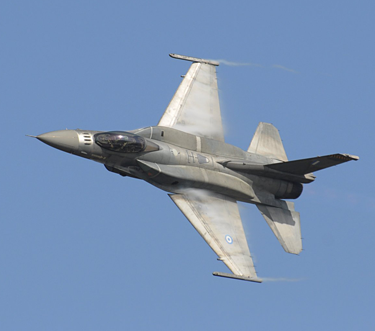
Original Plane |

Low Frequencies Plane |
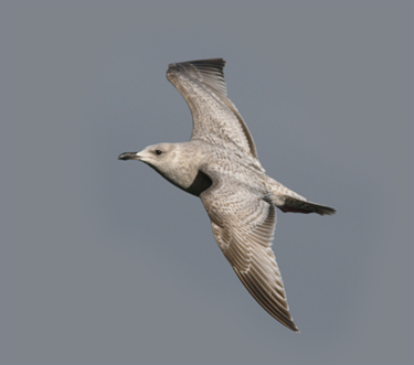
Original Bird |
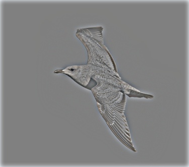
High Frequencies Bird |
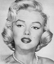
Original Marilyn |
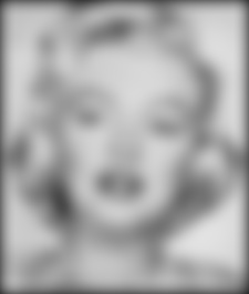
Low Frequencies Marilyn |
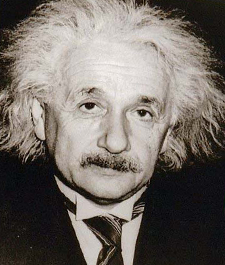
Original Einstein |
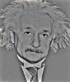
High Frequencies Einstein |
For the following image I changed my cutoff_frequency to 6.
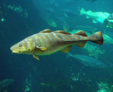
Original Fish |
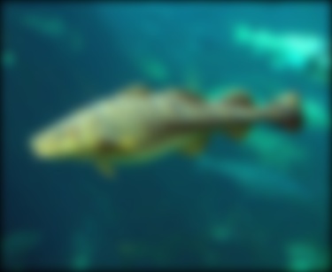
Low Frequencies Fish |
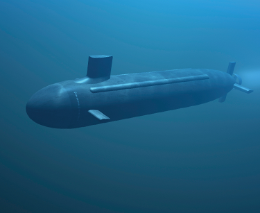
Original Submarine |
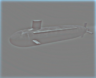
High Frequencies Submarine |
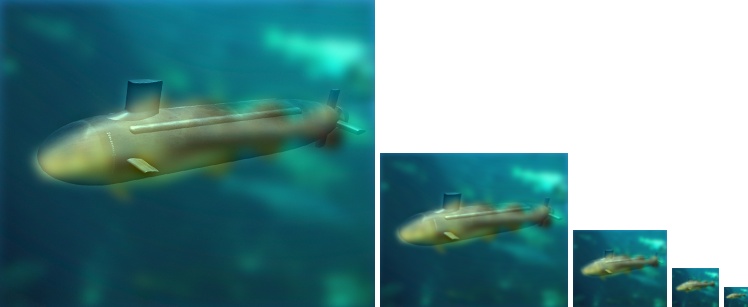
Note that the image results are different depending on which image we choose to do a low pass on and which image we choose to do a high pass on. As we can see we have created some interesting hybrid images which obey the properties we initially expected based on which image we performed a low pass on and which image we performed a high pass on!