Project 1: Image Filtering and Hybrid Images
For this project, I implemented an implementation of image filtering called my_imfilter and used that image filter to create hybrid images.
Image Filtering
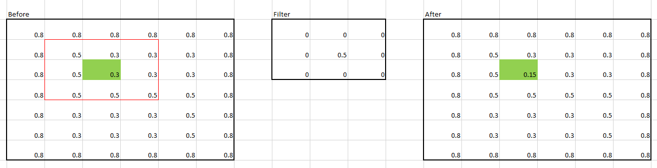
The image filtering algorithm was mainly done by looping through every pixel in the image that was being filtered, and then applying a given filter to that pixel. The filter was applied by identifying the section of the image centered around the current pixel being examined of the same size of the filter. Then, by adding up the results of doing element-wise multiplication between the section of the image previously identified for the current pixel and the given filter, the new resulting value for the current pixel was then determined and could be placed into the same position into a new matrix, which would store the resulting filtered image. This process was repeated for all remaining pixels in the current image, and in all three color channels. The three color channels were then combined in the third dimension as the same matrix, which could then be displayed as a regular image by MATLAB. An example of this technique is shown below, where the pixel at coordinate (3, 3) is being filtered by a 3 by 3 filter.
for i = 1:imageDepth
    for j = 1 + pv:imageRows + pv
        for k = 1 + ph:imageColumns + ph
            imageSection = finalChannels(j-pv:j+pv, k-ph:k+ph, i);
            result = sum(sum(imageSection .* filter));
            outputMatrix(j-pv, k-ph, i) = single(result);
        end
    end
end
The code above is where the filter is applied to all pixels in all channels in the image. pv and ph stand for padding vertical and padding horizontal, respectively.
The pixels near the border, however, posed another problem. Since the size of the filter generally considers various pixels around the current pixel being identified, many pixels on or near the border (depending on the size of the filter of course) could not yet have a filter applied to them, since there are no existing values around the pixels. For example, consider a pixel in the (2, 2) coordinate position being filtered by a (5, 5) size filter. This means that the filter, when applied to that coordinate, would need to identify values of pixels that do not exist in the image. A diagram of this scenario is shown below.

Notice how the 5 by 5 filter goes off the image where there are no values.
In order to resolve this problem, the image must be padded around the edges. The amount of padding necessary is half the size of the given filter being applied, rounded down. This is because the filter is centered on the pixel being examined, which leaves at most half of the filter rounded down that could happen to fall off the edges of the image. There are various techniques for padding the image. One way would be to simply give all padded pixels a value of zero. This solution is quickly achievable by using MATLAB's padarray() function, but leaves a distinct dark border or darkening effect on the edges of the resulting image in various filtering attempts. Thus, I instead mirrored the image on the edges to remove the darkening effect. By mirroring the image along the edges as padding, very similar colors and values to the current ones being used on the edges will be applied during the filter, thus allowing the padding to blend in with the rest of the image. This technique allows for a much less intrusive padding approach than simply padding the original image with all zero values.
top = channel(1:pv,:);
bottom = channel(size(channel, 1) - pv + 1:size(channel, 1),:);
channel = cat(1, flipud(top), channel, flipud(bottom));
The edges have been mirrored, which makes the new padding blend in with the rest of the image. An example snippet of code used to mirror the top and bottom of the images is also included. pv stands for padding vertical, and is calculated by taking the height of the filter divided by two rounded down.
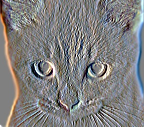
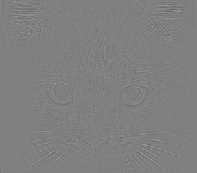
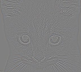
The results of the myfilter function with several sample filters is shown below. The first row contains the identity (original) image, blurred, and large blur in respective order. The second row contains the sobel filter, high pass filter, and laplacian filter in respective order.


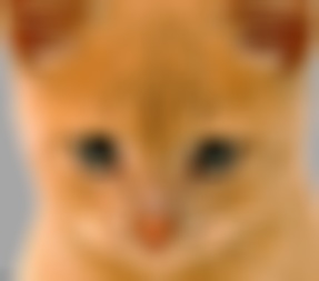
Here is one more example, with the original cat image, with the filters in the same order as the previous example.

Hybrid Images
The filtering function written previously was then used to produce hybrid images. The hybrid image is produced by combining (adding) two images together, but the two images must be filtered first for best results. One image will be high-pass filtered while the other image will be low-pass filtered. A low-pass filtered version of an image can be obtained by applying a Gaussian blur with some value of standard deviation, which determines how much high frequency to remove in this image. A high-pass filtered version of an image can be obtained by taking the original image and subtracting from it a low-pass filtered version of the same image with some value of standard deviation. This standard deviation is also known as cutoff-frequency, and must be fine-tuned manually in this case for optimal results. Some examples of hybrid images generated are shown below.
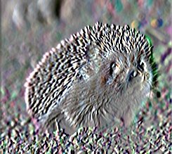
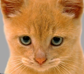
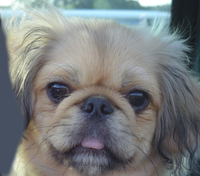
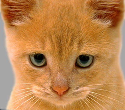
Below are the two original images used for producing the hybrid image. It's a picture of a dog, and another picture of a cat.
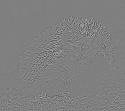
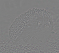
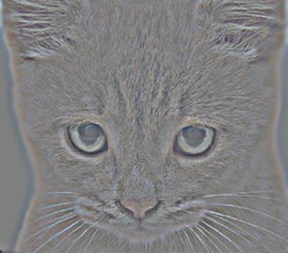
The high frequences from the dog image was then removed, and the low frequencies of the cat image was removed. The cutoff frequency used in this case was 7. These are shown below.

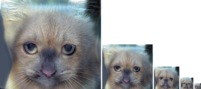
The final hybrid picture produced is shown below, in varying dimensions.
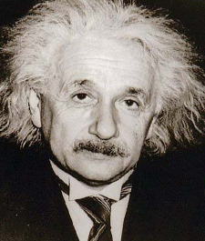
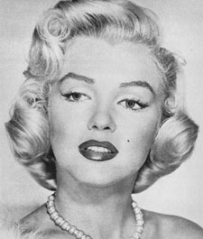
Next, the same code was used to combine a picture of Albert Einstein and Marilyn Monroe. Below are the two original images used for producing the hybrid image.
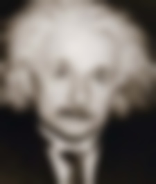
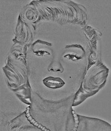
The high frequences from the Einstein image was then removed, and the low frequencies of the Marilyn image was removed. The cutoff frequency used for Einstein was 6, while the cutoff frequency used for Monroe was 4. These are shown below.
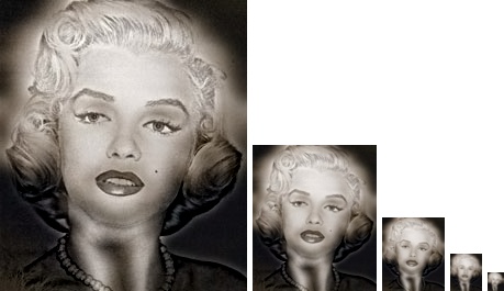
The final hybrid picture produced is shown below, in varying dimensions. Notice how from a smaller image (farther away), the image looks more like Albert Einstein, but close up, it looks more like Marilyn Monroe.
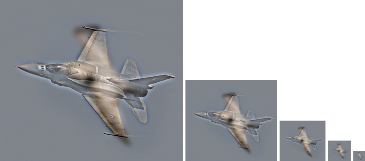
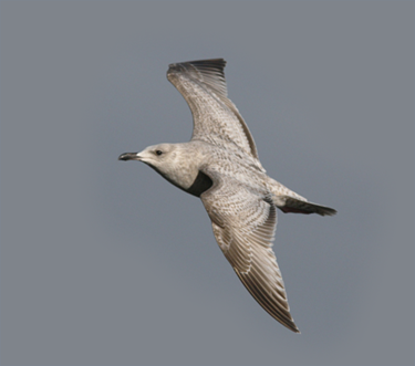
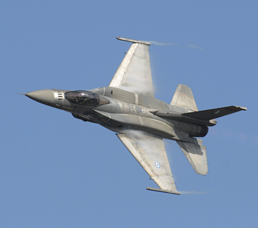
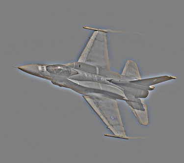
Finally, the same code was used to combine a picture of a bird and a plane. Below are the two original images used for producing the hybrid image.
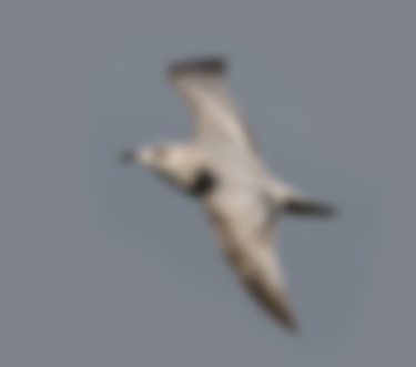
The high frequences from the bird image was then removed, and the low frequencies of the plane image was removed. The cutoff frequency used in this case was 5. These are shown below.
The final hybrid picture produced is shown below, in varying dimensions.