James Jonghan Park

Implementation of my_imfilter()

This image filtering process is done with convolution, where input image pixels are multiplied and added, a weighted average, with filter pixels known as a kernel.

function output = my_imfilter(image, filter)

[imgRow, imgCol, imgDepth] = size(image);

offset = size(filter) - 1;
padSize = ceil(offset/2);
output = zeros(size(image));

paddedImg = padarray(image, padSize, 'symmetric');

for z = 1:imgDepth
    for y = 1:imgRow
        for x = 1:imgCol
           output(y, x, z) = ...
               sum(sum(paddedImg(y:y+offset(1),x:x+offset(2), z).*filter));
        end
    end
end

Implementation clarifications

	
for z = 1:imgDepth
    for y = 1:imgRow
        for x = 1:imgCol ...

We define graphical image in matlab as arrays of doubles representing pixels, where color channels (ex. R,G,B) are represented with depth or z.

offset = size(filter) - 1;
...
paddedImg(y:y+offset(1),x:x+offset(2), z)

Matlab can retrieve a patch of pixels or subarray with :, where 1:3 shows range from 1 to 3 inclusive. We subtract offset by one to seamlessly match paddedImg size with filter size during operation below.

output(y, x, z) = ...
               sum(sum(paddedImg(y:y+offset(1),x:x+offset(2), z).*filter));

Note that we use paddedImg, and not the original image for this calculation.

paddedImg = padarray(image, padSize, 'symmetric');

Because we apply the weighted average with filter onto image, the resulting image will be smaller by the respective y and x offset. To counter this, we pad the image and then apply the respective operations. I apply the symmetric reflection padding to reduce corner noise from filtering (subjective).

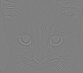
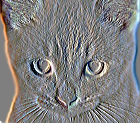
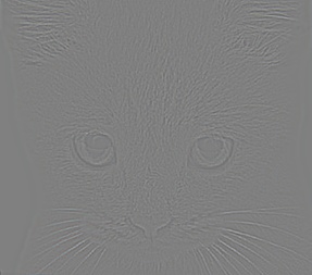
Results

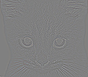
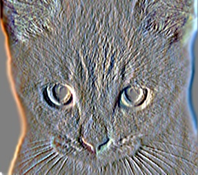
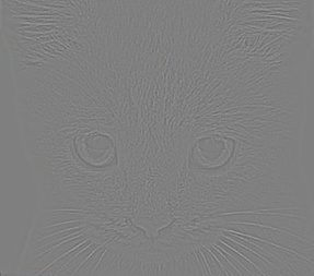
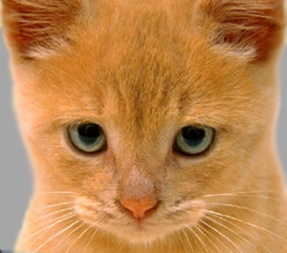
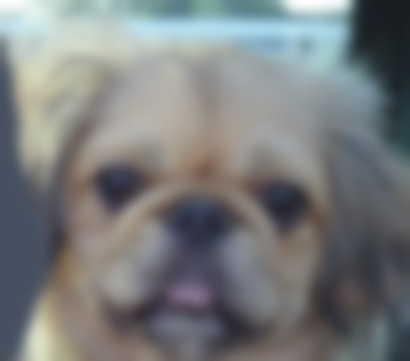
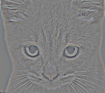
First row is the results from Mr. Park's my_imfilter implementation.
Second row is the results from imfilter of Matlab implementation.

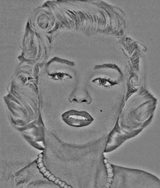
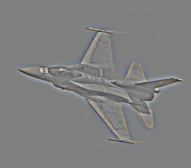
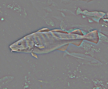
Applied filters from left to right:
identity, blur (box), large blur, (Gaussian) high pass (discrete Laplacian), oriented (Sobel operator), high pass (low freq subtraction)

The results from my implementation matches the matlab output with 'symmetric' optional parameter.

Implementation of proj1()'s filtering and hybrid image construction

Hybrid image is constructed by summing a low-pass filtered version of one image with a high-pass filtered version of another image. One way to accomplish a low-pass filter is by removing high frequencies through Gaussian filter with my_imfilter. Then a high-pass filter can be achieved by subtracting the original image against Gaussian filtered image. Alternatively, it appears that we can achieve this through discrete Laplacian (shown in proj1_test_filtering.m).
Below, I utilize a Gaussian blur filter.

filter = fspecial('Gaussian', cutoff_frequency*4+1, cutoff_frequency);
%%%%%%%%%%%%%%%%%%%%%%%%%%%%%%%%%%%%%%%%%%%%%%%%%%%%%%%%%%%%%%%%%%%%%%%%
% Remove the high frequencies from image1 by blurring it. The amount of
% blur that works best will vary with different image pairs
%%%%%%%%%%%%%%%%%%%%%%%%%%%%%%%%%%%%%%%%%%%%%%%%%%%%%%%%%%%%%%%%%%%%%%%%

low_frequencies = my_imfilter(image1, filter); 

%%%%%%%%%%%%%%%%%%%%%%%%%%%%%%%%%%%%%%%%%%%%%%%%%%%%%%%%%%%%%%%%%%%%%%%%
% Remove the low frequencies from image2. The easiest way to do this is to
% subtract a blurred version of image2 from the original version of image2.
% This will give you an image centered at zero with negative values.
%%%%%%%%%%%%%%%%%%%%%%%%%%%%%%%%%%%%%%%%%%%%%%%%%%%%%%%%%%%%%%%%%%%%%%%%

high_frequencies = image2 - my_imfilter(image2, filter);

%%%%%%%%%%%%%%%%%%%%%%%%%%%%%%%%%%%%%%%%%%%%%%%%%%%%%%%%%%%%%%%%%%%%%%%%
% Combine the high frequencies and low frequencies
%%%%%%%%%%%%%%%%%%%%%%%%%%%%%%%%%%%%%%%%%%%%%%%%%%%%%%%%%%%%%%%%%%%%%%%%

hybrid_image = low_frequencies + high_frequencies; 

Notice cutoff_frequency parameter.
Hybrid image requires this parameter, for each image set, to be tuned for good results as it represents a standard deviation of the Gaussian blur. This means that it dictates how much high and low frequencies should be kept for respective images.

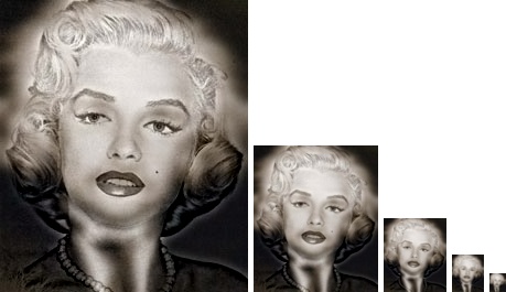
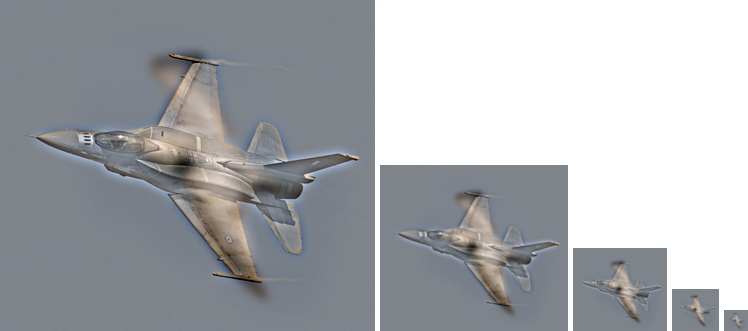
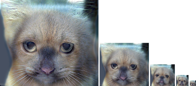
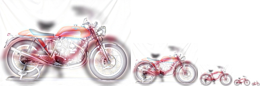
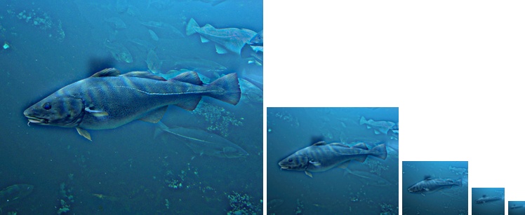
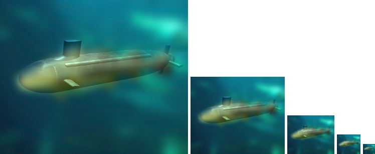
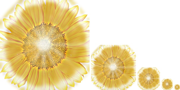
Results

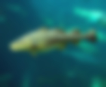
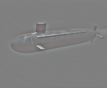
odd images = low-frequency images (Gaussian blur),
even images = high-frequency images,
Low to high cutoff_frequency from left to right (4.5, 5, 5, 6, 7, 9 standard deviation respectively)
Lower cutoff_frequency means less Gaussian blur that favors accenting low frequency image over high frequency image.

You can note that choosing which image to perform low or high frequency filtering also dictates how well hybrid image is constructed (as shown above with fish and submarine example).

Extra credit?

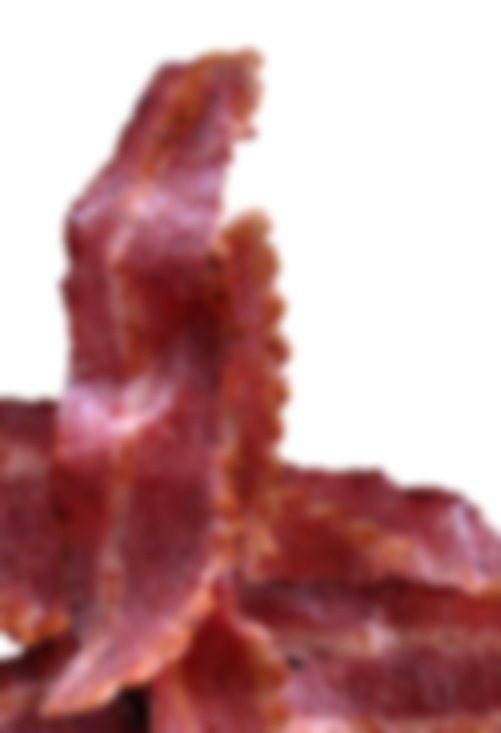
There's a saying that anything goes well with bacon...

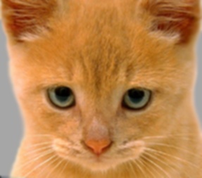
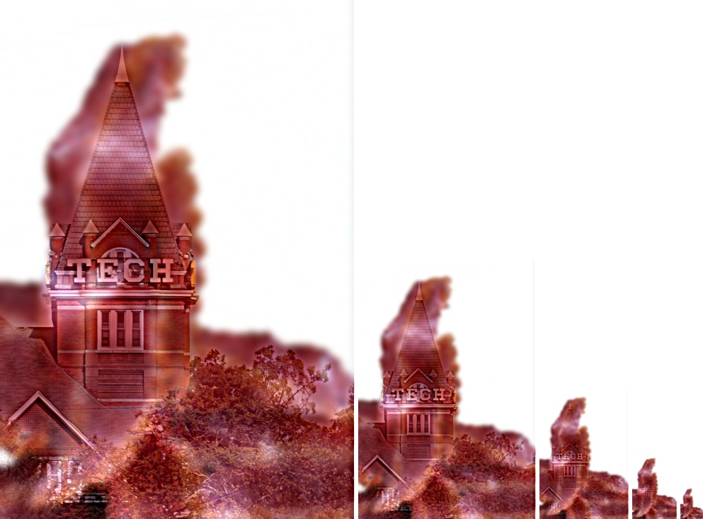
Another image for sanity.