Project 1: Image Filtering and Hybrid Images
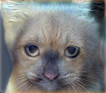
Fig. 1 A typical hybrid image made of a cat image and a dog image.
The objective of this project is to create hybrid images by using the simplified version of the method presented by Oliva, Torralba, and Schyns in SIGGRAPH 2006. The interpretation of hybrid images varies by the viewing distance. A typical hybrid image is shown in Fig. 1, which looks like a cat or a dog when the viewing distance is close or far, respectively.
Method
The method used in this project includes three steps: 1) Selecting two images and tailoring them to the same dimension for perfect alignment; 2) Processing the two tailored images using low-pass filter and high-pass filter, respectively; 3) Combining the two processed images to obtain the hybrid image. The low-pass filter is a Gaussian filter and the high-pass filter is constcuted by subtracting the low-frequency content, which is also obtained by the Gaussian filter, from the original image. Different cutoff frequcies for the two images are used to tune the hybrid image. In the process of image filtering, all the original images are padded with zeros or reflected image content around their edges.
Example of Code with Highlighting The example code is presented as follows. The padding size is decided by the dimension of filter, which is assumed to have an odd dimension. Most images are padded by default with zeros and padding with reflected image content is also tested for comparison. Then, iterations are run to calculate the value of each pixel in a blank image by applying the filter for each pixel in the orignal image.
%example code
Hpad=(Hfilter-1)*0.5; % pad height
Wpad=(Wfilter-1)*0.5; % pad width
Padimage=padarray(image,[Hpad Wpad]); % image padding around edges with zeros
%Padimage=padarray(image,[Hpad Wpad],'symmetric'); % image padding around edges with reflected content
for c=1:1:Channel
    for m=1:1:Himage
        for n=1:1:Wimage
            pixelvalue=0.0;
            for k=1:1:Hfilter
                for l=1:1:Wfilter
                    pixelvalue=pixelvalue+Padimage(m+k-1,n+l-1,c)*filter(k,l); % pixel value by applying the filter
                end
            end
            Bimage(m,n,c)=pixelvalue; % feed value to the blank image
        end
    end
end
Results and Discussion
The developed image filter is tested by applying several different filters. Figs. 2(a) and 2(b) show the orignal image and the result after applying the Indetify filter, respectively. Figs. 2(c) and 2(d) show the blurred images by applying a box filter and a Gaussian filter, respectively. Since we use zero padding, the edges of the blurred images are dark. When reflected image content is used for padding, this problem can be avoided, as shown in Fig. 2(e). Figs. 2(f) and 2(g) show the results when a Sobel filter and a discrete Laplacian filter are applied, respectively. Fig. 2(h) shows the high-frequncy content of the image by subtracting the low frequencies (Fig. 2(c)) from the original image.
(a)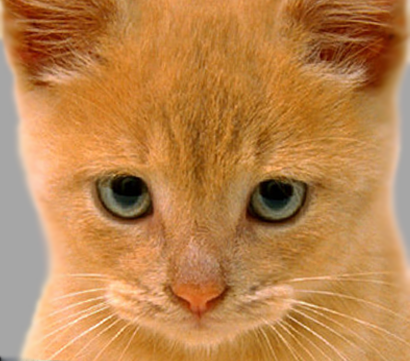 (b)
(b)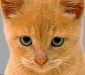 (c)
(c)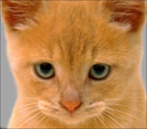 (d)
(d)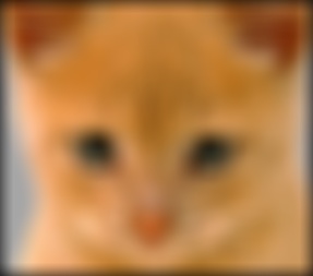
|
(e)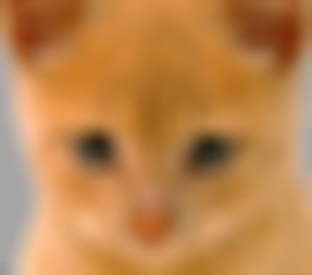 (f)
(f)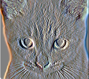 (g)
(g)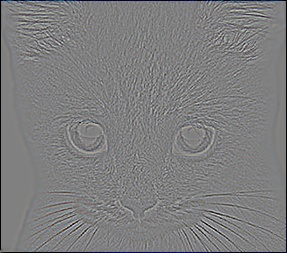 (h)
(h)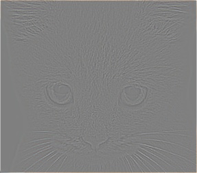
|
|
Fig. 2 (a) Original image of cat. (b) Identical image of cat using Identify filter. (c) Blurred image of cat using a box filter. (d) Largely blurred image of cat using Gaussian filter. (d) Largely blurred image of cat using Gaussian filter (Padding with reflected image content). (f) Processed image of cat using Sobel filter. (g) Processed image of cat using discrete Laplacian filter. (h) High-frequency image of cat by subtracting the low-frequency content. |
The hybrid images are generated based on pairs of different images as shown in Figs. 3 to Figs. 8. The cutoff frequencies are tuned to obtain the best illusion effect. It is found that if the pair of images have the similar color, the high-frequency content can be more obvious in close distance, since the viewer will not be distracted by the low-frequency content due to the color. The examples are given by Figs. 3 and 8.
(a) (b)
(c)
(b)
(c)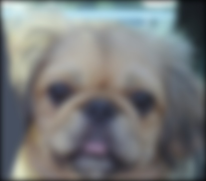 (d)
(d)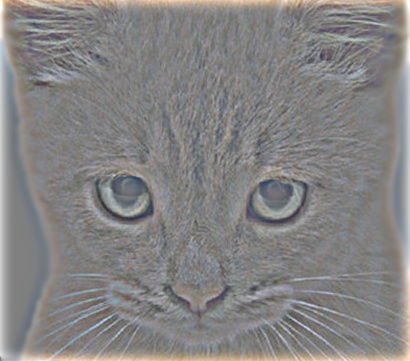
|
(e)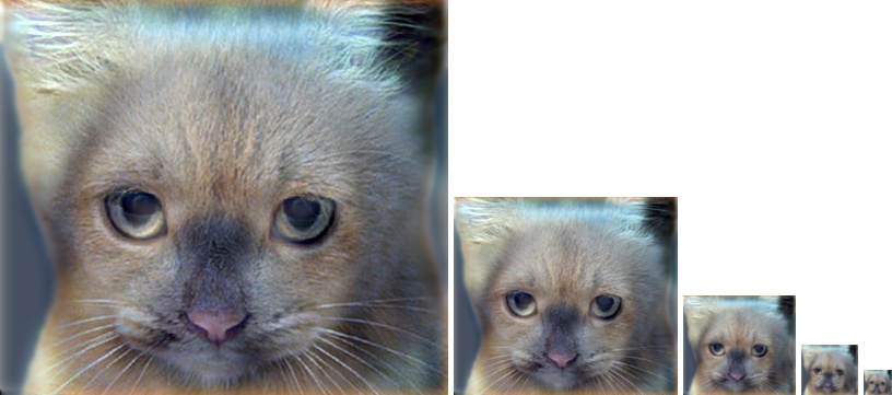
|
|
Fig. 3 (a) Original image of dog. (b) Original image of cat. (c) Low-frequency image of dog (fcutoff = 7). (d) High-frequency image of cat (fcutoff = 7). (e) Hybrid image with different scales. |
(a)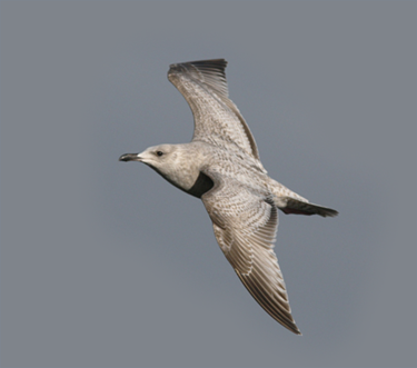 (b)
(b)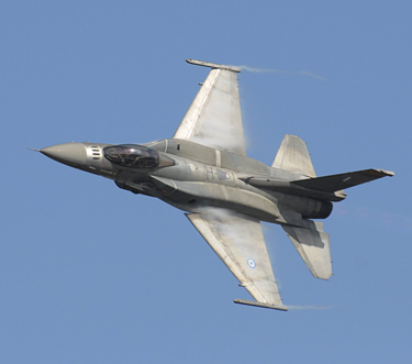 (c)
(c)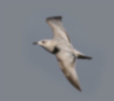 (d)
(d)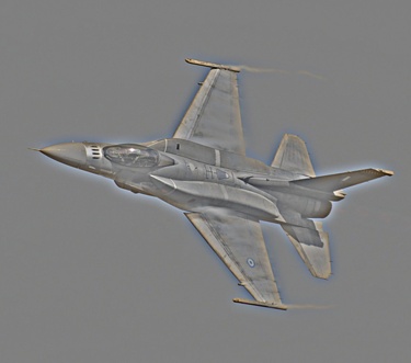
|
(e)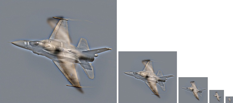
|
|
Fig. 4 (a) Original image of bird. (b) Original image of plane. (c) Low-frequency image of bird (fcutoff = 3). (d) High-frequency image of plane (fcutoff = 5). (e) Hybrid image with different scales. |
(a)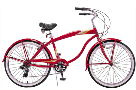 (b)
(b)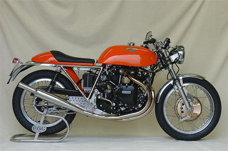 (c)
(c)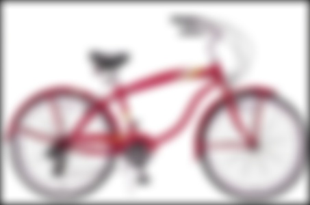 (d)
(d)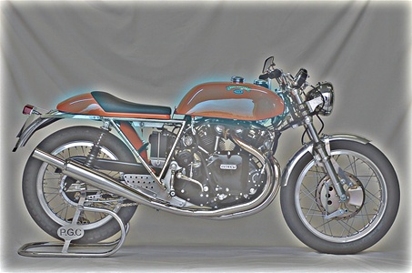
|
(e)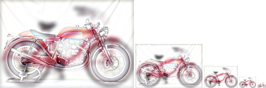
|
|
Fig. 5 (a) Original image of bicycle. (b) Original image of motorcycle. (c) Low-frequency image of bicycle (fcutoff = 7). (d) High-frequency image of motorcycle (fcutoff = 7). (e) Hybrid image with different scales. |
(a)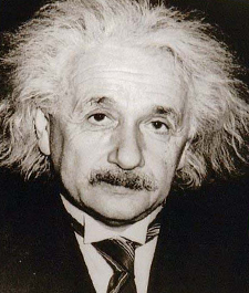 (b)
(b)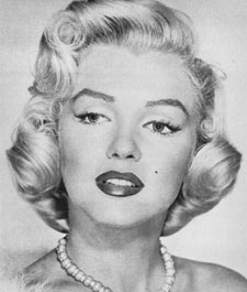 (c)
(c)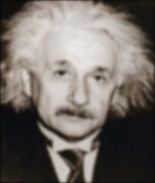 (d)
(d)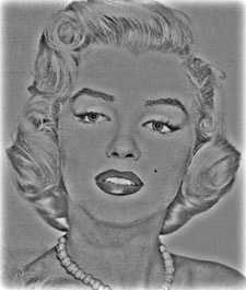
|
(e)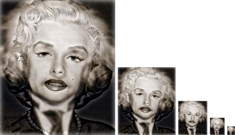
|
|
Fig. 6 (a) Original image of Einstein. (b) Original image of Marilyn. (c) Low-frequency image of Einstein (fcutoff = 2). (d) High-frequency image of Marilyn (fcutoff = 5). (e) Hybrid image with different scales. |
(a)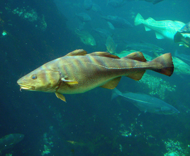 (b)
(b)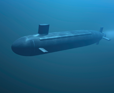 (c)
(c)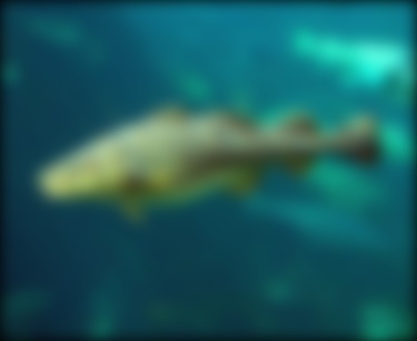 (d)
(d)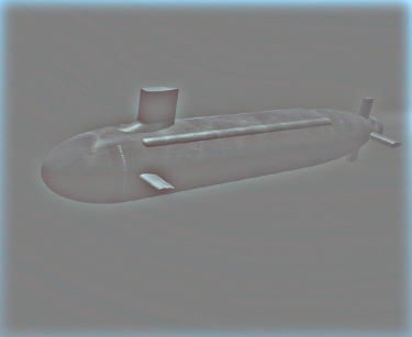
|
(e)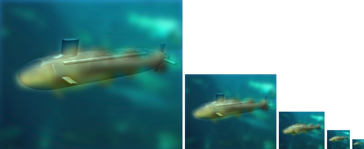
|
|
Fig. 7 (a) Original image of fish. (b) Original image of submarine. (c) Low-frequency image of fish (fcutoff = 7). (d) High-frequency image of submarine (fcutoff = 7). (e) Hybrid image with different scales. |
(a)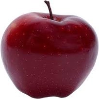 (b)
(b)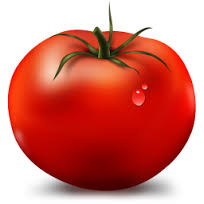 (c)
(c)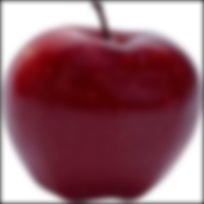 (d)
(d)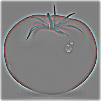
|
(e)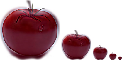
|
|
Fig. 8 (a) Original image of apple. (b) Original image of tomato. (c) Low-frequency image of apple (fcutoff = 3). (d) High-frequency image of tomato (fcutoff = 3). (e) Hybrid image with different scales. |