Project 1: Image Filtering and Hybrid Images
The first part to creating hybrid images is to re-create matlab's imfilter function. To do this, there are three key aspects to consider.
- Following the algorithm
- What to do about the boundaries
- What to do about the colors
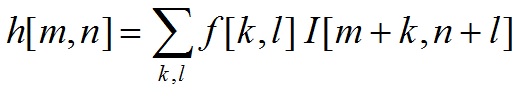
Filtering Algorithm
Filtering Algorithm
The filtering algorithm is displayed above. It says that for every element in the image, loop through the filter and multiply the corresponding elements. Then, sum them. To ensure the correct alignment of the filter and the image, I chose my main loop to be the desired position of the output pixel and then adjusted the image's pixel index according to the filter's size. The adjustment is shown below.
    imagerow = row - (filterRows+1)/2 + i;
    imagecol = col - (filterCols+1)/2 + j;
What to do about the boundaries
We cannot use the algorithm to compute the values at the borders due to a lack of input elements. There isn't an obvious solution to the question of what to do with the borders. However, the instructions indicate to "(3) pad the input image with zeros or reflected image content". So I decided that padding with zeroes is the easily implemented option of the two. Rather than pre-processing the image to add a black border, I simply modified the algorithm to simulate the black border. This reduces the space and time complexity of the program.
To simulate the padding of zeros, I check to see if the image index I wish to use is within the bounds of the image. If it is, I act according to the algorithm. If it isn't, I continue to the next iteration.
What to do about the colors
The filter must "(1) support grayscale and color images". So this means that the input image can either be a 2d or 3d matrix. It is possible to see 2d matrixes as 3d matrices with a size one 3rd dimension. So, to ensure I capture all colors of the image, I added another loop to iterate over all the colors. A greyscale image will simply undergo a single iteration and preceed as normal.
The final code
for color=1:1:size(image,3) %color, 3 for rgb, 1 for greyscale
    for row=1:1:imageRows %row
        for col=1:1:imageCols %col

            tempSum = 0;
            for i=1:1:filterRows
                for j=1:1:filterCols
                    imagerow = row - (filterRows+1)/2 + i;
                    imagecol = col - (filterCols+1)/2 + j;
                    if (imagerow>0 && imagerow<=imageRows && ...
                            imagecol>0 && imagecol<=imageCols)%both row and col are in bounds
                        product = filter(i,j) * image(imagerow,imagecol,color);
                        tempSum = tempSum + product;
                    end
                end
            end
            output(row, col, color) = tempSum;

        end
    end
end
Results from testing my_imfilter
I tested my code with the p=test script provided to get the following results. From left to right, the image is blur, high pass, identity, laplacian, large blur, and sobel. With these results, I assumed that the filter was working as intended.
|
|
Hybrid Image
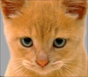
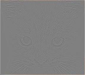
Now that the filter is working, it's trivial to set up the hybrid image. To generate the low-pass image, a gaussian blur is applied as a filter. To generate the high-pass image, the same blur is applied but then subtracted from the original image. The hybrid image is the sum of the two images. The code is provided below.
low_frequencies = my_imfilter(image1, filter)
high_frequencies = image2 - my_imfilter(image2, filter)
hybrid_image = low_frequencies + high_frequencies
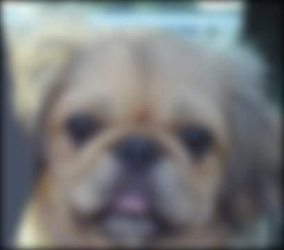
Once that was implemented, it's time to test the hybrid image. Using the images provided, I get the following results.
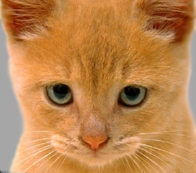
| Original images | |

|

|
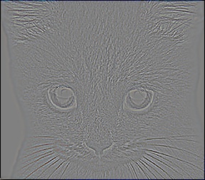
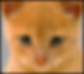
| Filtered images | |
| Low-Pass | High-Pass |
|
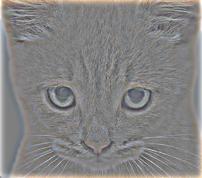
|
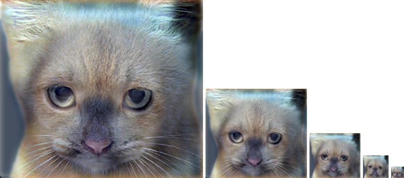
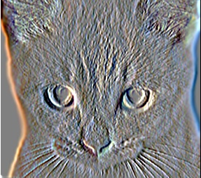
| Hybrid image | |
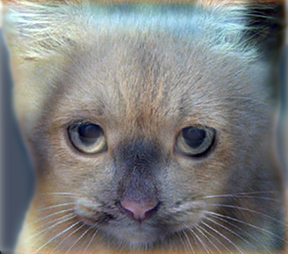
|
|
| Image Scales |