Project 1: Image Filtering and Hybrid Images
Image Filtering algorithm
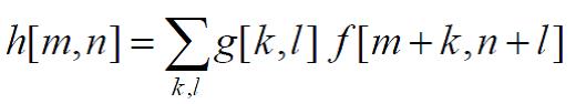
For a 2D filter, g[.,.], and an image, f[.,.], the resultant filtered image, h[.,.], can be obtained by the formular of:
Process Flow
- Make RGB channels to be individual if the input image is colored.
- Check filter size (assumed odd size only).
- Define computation area.
- Calculate the convolution with zero-padding.
- Return the output value.
Code for my_imfilter
function output = my_imfilter(image, filter)
%%%%%%%%%%%%%%%%
% Your code here
%%%%%%%%%%%%%%%%
imgSize = size(image);
output = zeros(imgSize);
tempSize = size(imgSize);
if tempSize(end) > 2 %for color image, handling layer by layer (assume that there is either grey or RGB color image)
    for i = 1:imgSize(3)
        output(:, :, i) = my_imfilter(image(:, :, i), filter);
    end
else
    [fil_h, fil_w] = size(filter); %check filter size (assume for only odd size of filter)
    h = round(fil_h/2);
    w = round(fil_w/2);
    for x = 1:imgSize(1)
        for y = 1:imgSize(2)
            %Definiing Upper/Lower limitations of the calculation area with ignoring the edge which corresponds with zero padding
            xL = min(h-1, x-1);
            xU = min(h-1, imgSize(1) - x);
            yL = min(w-1, y-1);
            yU = min(w-1, imgSize(2) - y);

            %Caculation for the output
            output(x, y) = sum( sum( image(x-xL:x+xU, y-yL:y+yU).* filter(h-xL:h+xU, w-yL:w+yU) ) );
        end
    end
end
Results of image filtering
Identity Filtered Image.
Blured Image.
Large Blured Image.
Sobel Filtered Image.
Laplacian Filtered Image.
High Pass Filtered Image.
Hybrid Image
Using the formular, H = I1*G1 + I2*(1-G2) where I1 and I2 is a input image filtered by low pass filter G1 and by high pass filter (1-G2), respectiveley, while H is the resultant hybrid image.
Considered only one cut-off frequency (i.e. G1=G2) and tuned the frequency for each pair of images, several hybrid images can be obtained as below.
Code for generating hybrid image
%% Setup
% read images and convert to floating point format
pairNum=1; %change 1 to 5 to select a pair of images
imagenames={'dog', 'cat'; 'bicycle', 'motorcycle'; 'bird', 'plane'; 'einstein', 'marilyn'; 'fish', 'submarine'};
dir='C:\Users\Kihan.Park\Desktop\Kihan\3)Course Work\2016 Fall\CS6467 Computer Vision\Project\1\proj1\data\';
for i=1:size(imagenames,2)
eval(sprintf('image%d=im2single(imread(''%s%s.bmp''));',i,dir,char(imagenames(pairNum,i))));
end

%% Filtering and Hybrid Image construction
cutoff_frequency = 7;
filter = fspecial('Gaussian', cutoff_frequency*4+1, cutoff_frequency);
low_frequencies = my_imfilter(image1,filter);
high_frequencies = image2-my_imfilter(image2,filter);
hybrid_image = low_frequencies + high_frequencies;

%% Visualize and save outputs
figure(1); imshow(low_frequencies)
figure(2); imshow(high_frequencies + 0.5);
vis = vis_hybrid_image(hybrid_image);
figure(3); imshow(vis);
imwrite(low_frequencies, 'low_frequencies.jpg', 'quality', 95);
imwrite(high_frequencies + 0.5, 'high_frequencies.jpg', 'quality', 95);
imwrite(hybrid_image, 'hybrid_image.jpg', 'quality', 95);
imwrite(vis, 'hybrid_image_scales.jpg', 'quality', 95);
Results of Hybrid Image
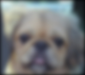
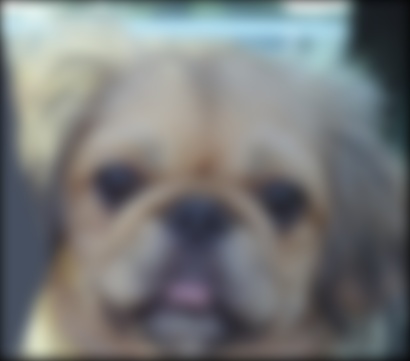
Low pass filtered "Dog".
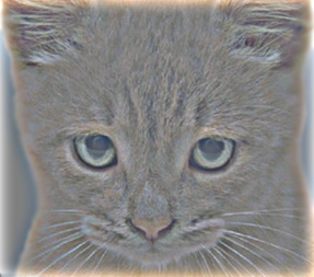
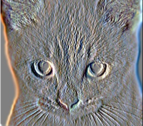
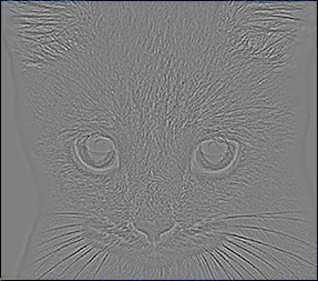
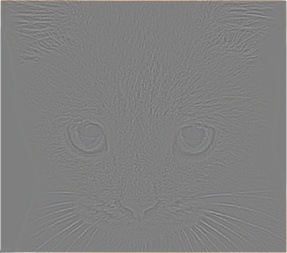
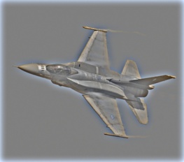
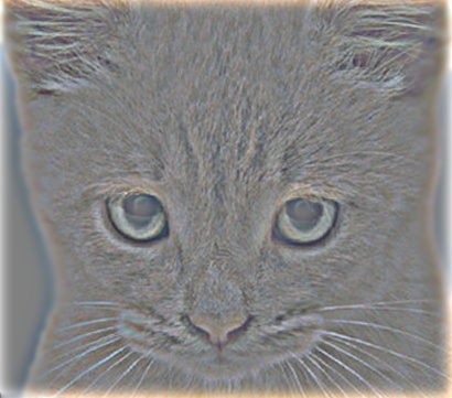
High pass filtered "Cat".
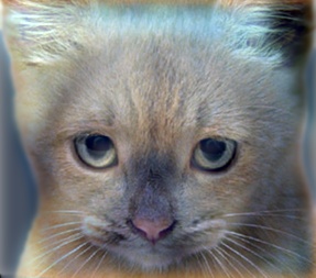
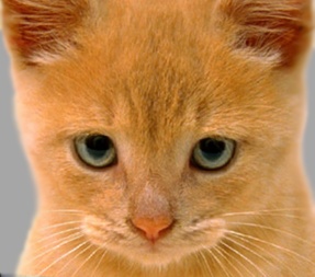
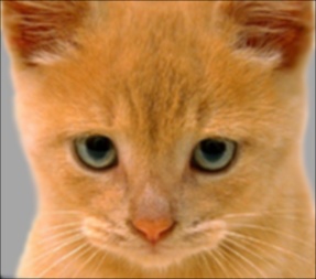
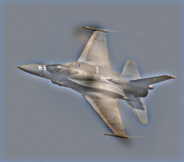
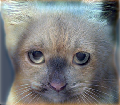
Hybrid image (Cut-off freq. : 7).
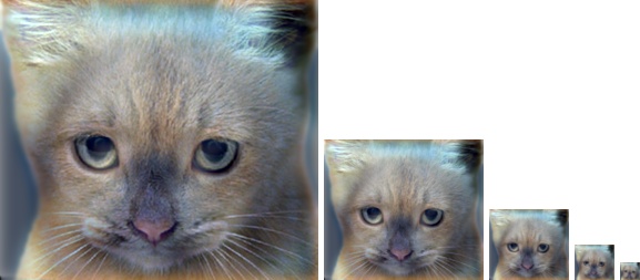
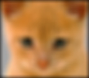
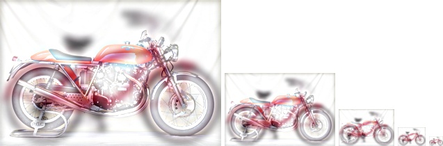
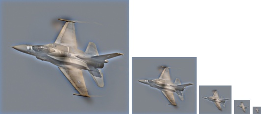
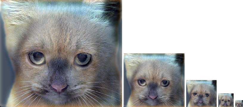
Scaled hybrid image.
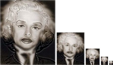
When we scale the hybrid image down, we can see the low pass filtered image (dog in this case) more clearly. It is becuase of down sampling (i.e. reducing resolution) has an effect of losing high frequency part of the image.
Other Results in a table
|
|
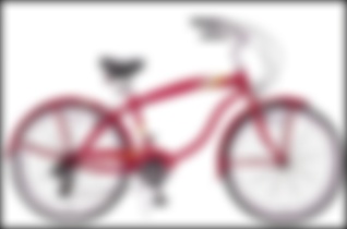
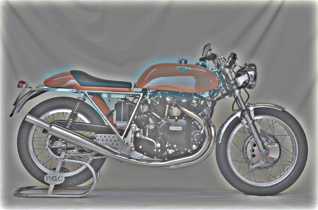
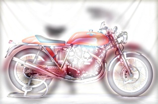
Low pass filtered "Bicycle" + High pass filtered "Motorcycle" (cut-off freq. : 5) |
|
|
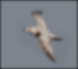
Low pass filtered "Bird" + High pass filtered "Plane" (cut-off freq. : 5) |
|
|
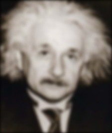
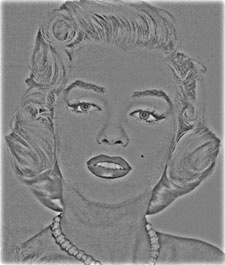
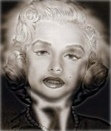
Low pass filtered "Einstein" + High pass filtered "Marilyn" (cut-off freq. : 3) |

|
|
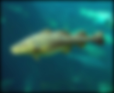
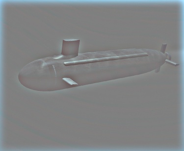
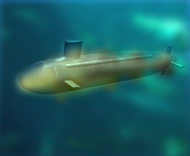
Low pass filtered "Fish" + High pass filtered "Submarine" (cut-off freq. : 8) |
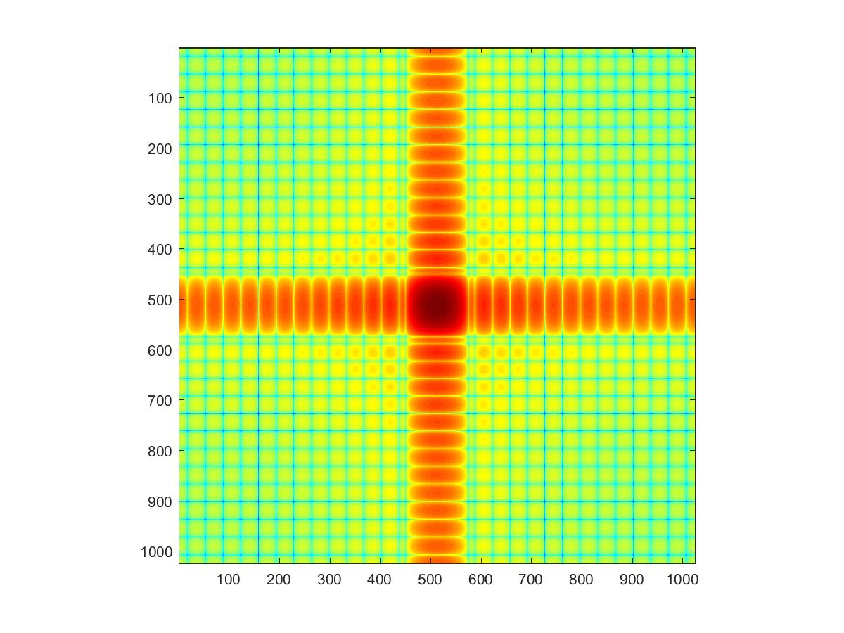
Extra Credit : Hybrid Image with FFT
Convolution in spatial domain is equivalent to multiplication in frequency domain. Therefore, instead of filtering with spacial convolution, we can do same job in frequency domain with FFT.
Process Flow
- Make RGB channels to be individual if the input image is colored.
- Check filter size (assumed odd size only).
- Define frequency range in order of 2 including padding.
- FFT image.
- Pad filter to be same size as image and FFT filter.
- Multiply image by filter elementwise.
- Inverse FFT image.
- Remove padding and return the ouput.
Code for FFT
function [output, im_fft, fil_fft] = my_imfilter_fft(image, filter)
%%%%%%%%%%%%%%%%
% Your code here
%%%%%%%%%%%%%%%%
imgSize = size(image);
output = zeros(imgSize);
tempSize = size(imgSize);
if tempSize(end) > 2 %for color image, handling layer by layer (assume that there is either grey or RGB color image)
for i = 1:imgSize(3)
[output(:, :, i),im_fft(:,:,i),fil_fft(:,:,i)] = my_imfilter_fft(squeeze(image(:, :, i)), filter);
end
else
[fil_h, fil_w] = size(filter); %check filter size (assume for only odd size of filter)
h = round(fil_h/2);
w = round(fil_w/2);
fftsize= 1024; % should be order of 2 (for speed) and include padding
im_fft = fft2(image, fftsize, fftsize); % fft im with padding
fil_fft= fft2(filter, fftsize, fftsize); % fftfil, pad to same size as image
im_fil_fft = im_fft .* fil_fft; % multiply fft images
im_fil = ifft2(im_fil_fft); % inverse fft2
im_fil = im_fil(1+h:size(image,1)+h, 1+h:size(image, 2)+h); % remove padding
output = im_fil;
end
%%%%%%%%%%%%%%%%%%%%%%%%%%%%%%%%%%%%%%%%%%%%%%%%%%
%% Filtering and Hybrid Image construction
cutoff_frequency = 7; %This is the standard deviation, in pixels, of the
filter = fspecial('Gaussian', cutoff_frequency*4+1, cutoff_frequency);
[low_frequencies,im1_fft,fil_fft] = my_imfilter_fft(image1,filter);
[low_frequencies2,im2_fft,fil_fft] = my_imfilter_fft(image2,filter);
high_frequencies=image2-low_frequencies2;
hybrid_image = low_frequencies + high_frequencies;
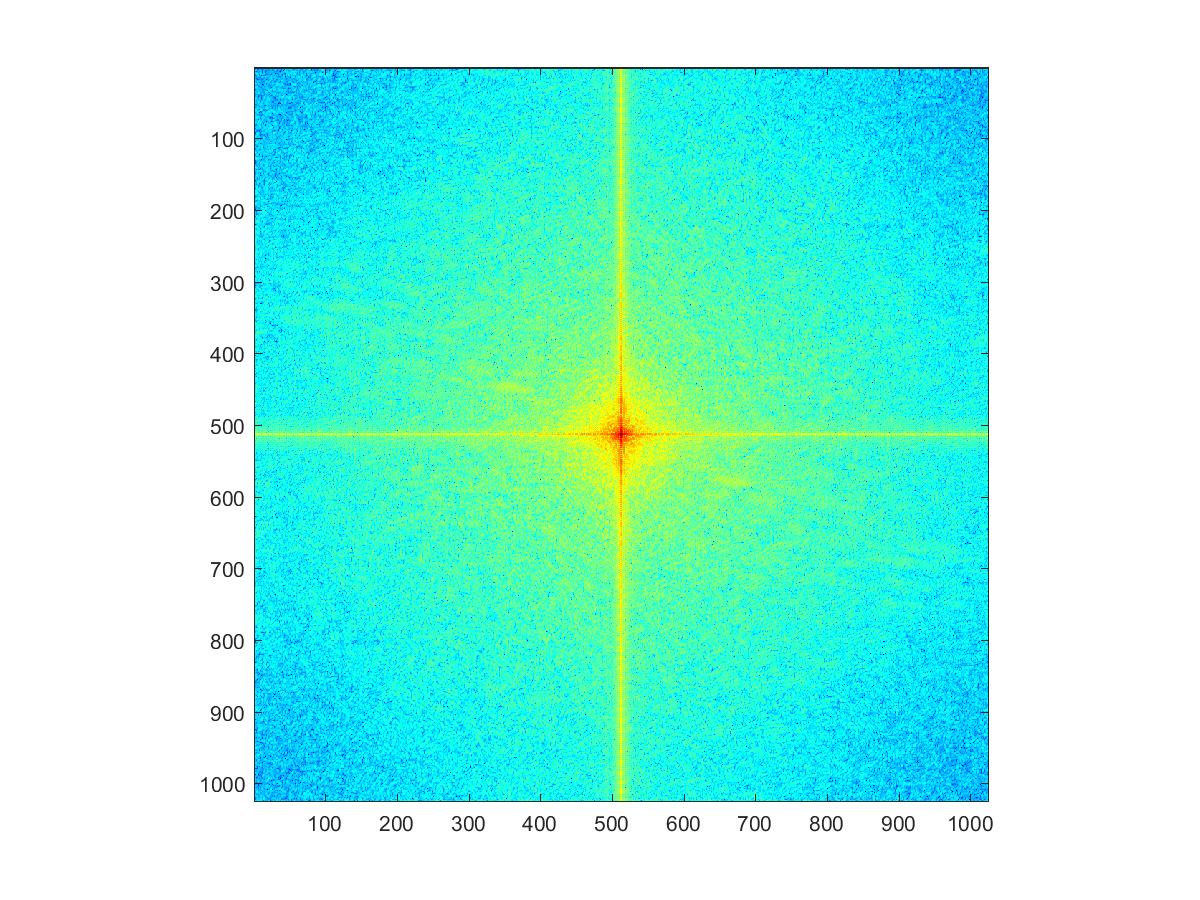
figure(1), im1_fft_R=imagesc(log(abs(fftshift(im1_fft(:,:,1))))), axis image, colormap jet
saveas(im1_fft_R,'image1_fft_R.jpg')
figure(2), im1_fft_G=imagesc(log(abs(fftshift(im1_fft(:,:,2))))), axis image, colormap jet
saveas(im1_fft_G,'image1_fft_G.jpg')
figure(3), im1_fft_B=imagesc(log(abs(fftshift(im1_fft(:,:,3))))), axis image, colormap jet
saveas(im1_fft_B,'image1_fft_B.jpg')
figure(4), im2_fft_R=imagesc(log(abs(fftshift(im2_fft(:,:,1))))), axis image, colormap jet
saveas(im2_fft_R,'image2_fft_R.jpg')
figure(5), im2_fft_G=imagesc(log(abs(fftshift(im2_fft(:,:,2))))), axis image, colormap jet
saveas(im2_fft_G,'image2_fft_G.jpg')
figure(6), im2_fft_B=imagesc(log(abs(fftshift(im2_fft(:,:,3))))), axis image, colormap jet
saveas(im2_fft_B,'image2_fft_B.jpg')
figure(7), fil_fft_R=imagesc(log(abs(fftshift(fil_fft(:,:,1))))), axis image, colormap jet
saveas(fil_fft_R,'filter_fft_R.jpg')
figure(8), fil_fft_G=imagesc(log(abs(fftshift(fil_fft(:,:,2))))), axis image, colormap jet
saveas(fil_fft_G,'filter_fft_G.jpg')
figure(9), fil_fft_B=imagesc(log(abs(fftshift(fil_fft(:,:,3))))), axis image, colormap jet
saveas(fil_fft_B,'filter_fft_B.jpg')
%% Visualize and save outputs
figure(10); imshow(low_frequencies)
figure(11); imshow(high_frequencies + 0.5);
vis = vis_hybrid_image(hybrid_image);
figure(12); imshow(vis);
imwrite(low_frequencies, 'low_frequencies.jpg', 'quality', 95);
imwrite(high_frequencies + 0.5, 'high_frequencies.jpg', 'quality', 95);
imwrite(hybrid_image, 'hybrid_image.jpg', 'quality', 95);
imwrite(vis, 'hybrid_image_scales.jpg', 'quality', 95);
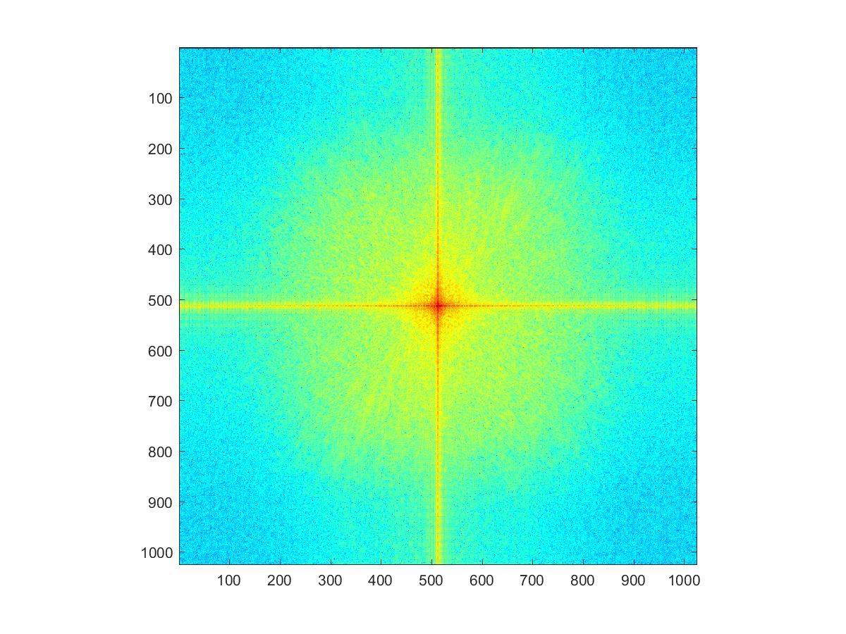
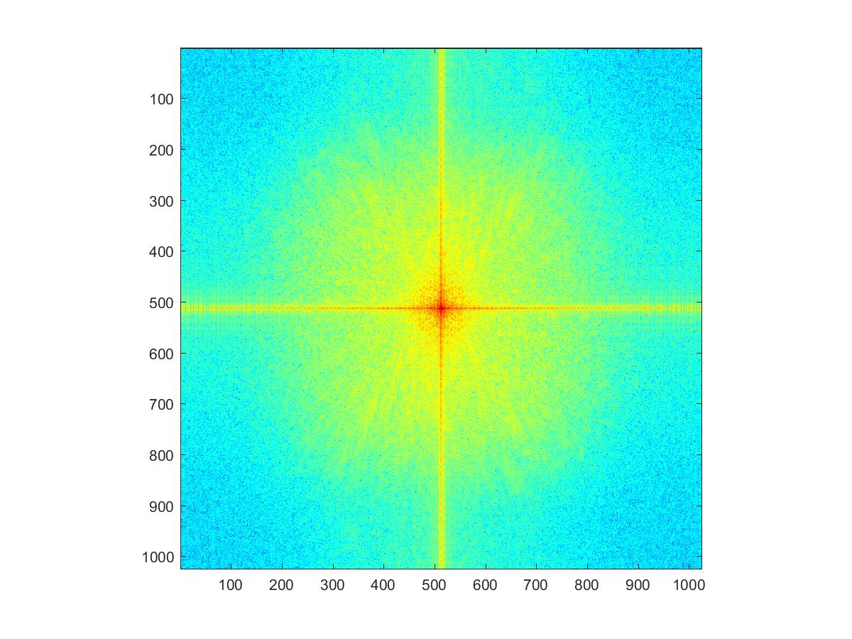
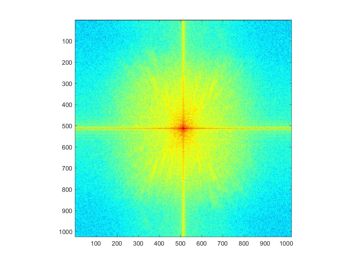
FFT Results in a table
|
|
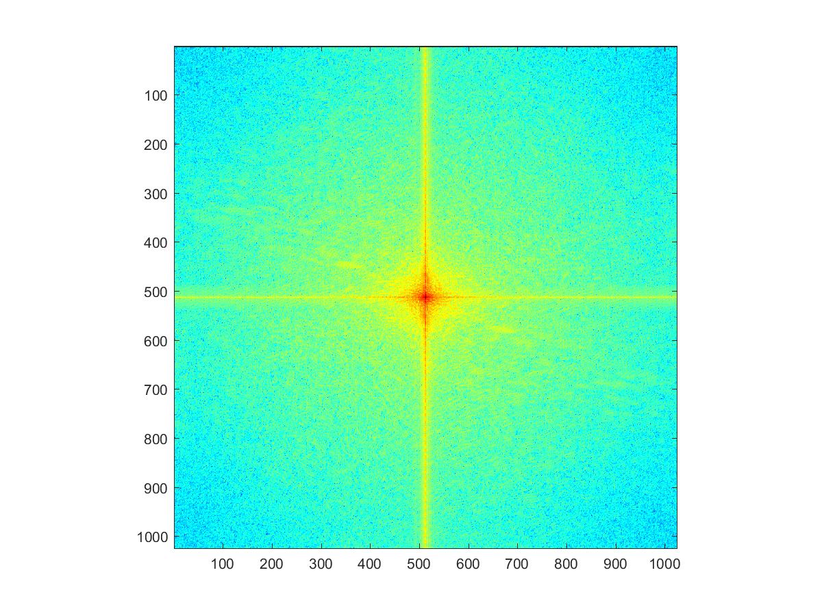
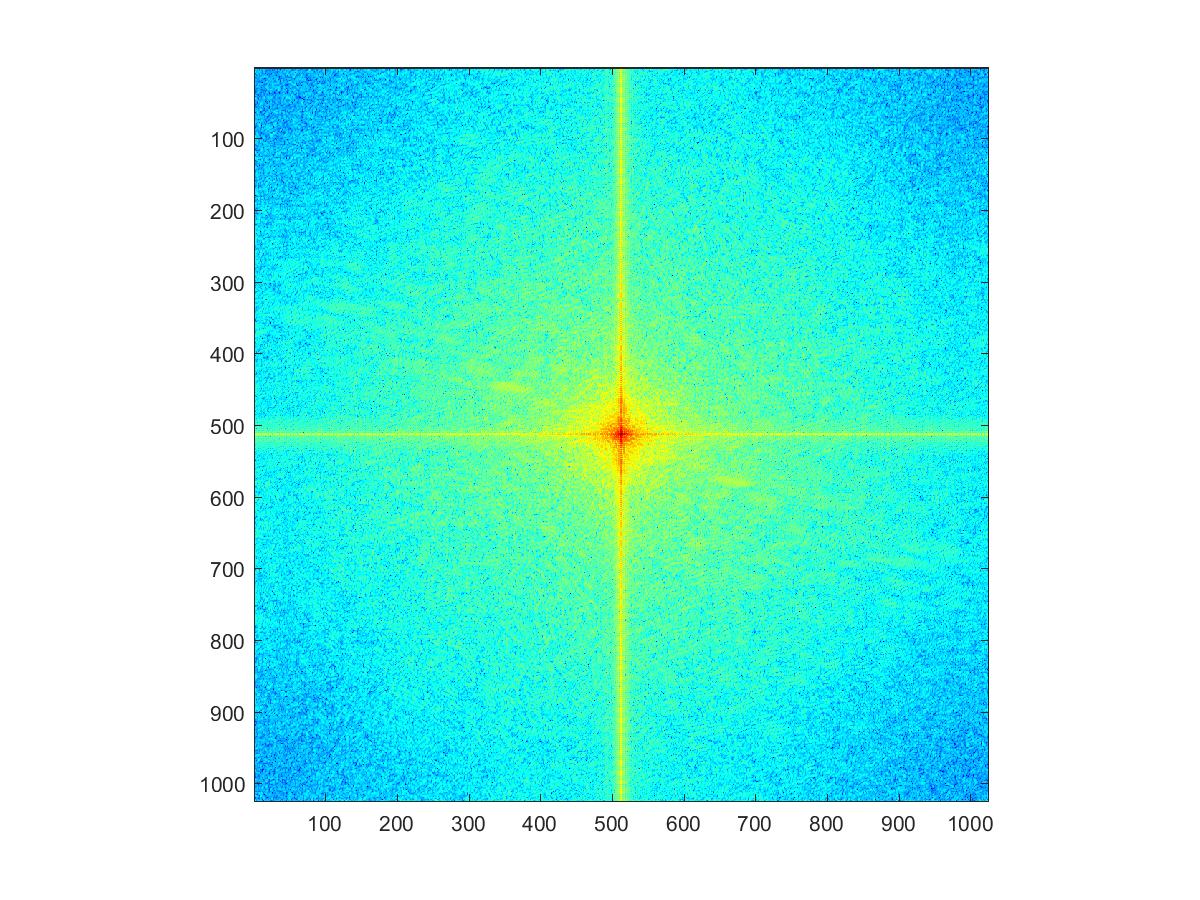
FFT of "Dog" from R,G, and B channel. |
|
|
FFT of "Cat" from R,G, and B channel. |


|
|
FFT of Gaussian low pass filter (cut-off freq. : 7) from R,G, and B channel. |
|
|
Hybrid image with FFT |
Through FFT and inverse FFT, we can obtain a hybrid image which is qualitatively same result with the filtering from spatial convolution.