Project 1: Image Filtering and Hybrid Images
The following writeup is organized as follows:
1. I have described the image filtering algorithm used along with the variants I have implemented and the results.
2. I have also compared the time taken for the varaints of the image filtering algorithm.
3. The procedure for the generation of hybrid images is outlined next.
4. I have also implemented image filtering in the frequency domain which is described below along with its results.
5. I have also tried experimenting the hybrid image generation with few other examples shown at the end.
Image Filtering algorithm
The algorithm initially creates an empty output array of the same dimension as that of the input image. Then for each pixel, the algorithm obtains a local neighborhood of that pixel from the original image and this is then multiplied (element-wise) with the filter matrix and the sum of the product result is taken to be the value for that particular pixel. This is computed for every pixel in the image and the final output i.e. the filtered image is stored in 'output' variable. I have implemented several variants of the filtering algorithm with respect to the boundary pixels and padding the image each of which I have discussed below along with the results.
Variant 1:
This is present in the file 'my_imfilter.m'. For the case of boundary pixels- the values for the local neighbourhood matrix of each pixel is obtained by using the pixels value from the input image for those which fall within the dimension of the input image and the rest of the values of the local matrix are assigned zero value. This is just a plain implementation of the filtering algorithm described above. padarray() function is not used here. Instead the idea is implemented.
	...
	...
            for ss1=1:s1 					%local matrix is contsructed here from the input image
                for ss2=1:s2
                    if i-p1+ss1<1 | i-p1+ss1>r | j-p2+ss2<1 | j-p2+ss2>c
                        local(ss1,ss2)=0;
                    else
                        local(ss1,ss2)=image(i-p1+ss1,j-p2+ss2,k);
                    end
                    %display(local(ss1,ss2));
                end
            end
    	...
    	...
Variant 2:
This is written in the 'my_imfilter2.m' file. In the case of boundary pixels- the local matrix is populated with the values in the input image for those cells of the matrix which fall within the dimension of the input image and their average is computed. Then, the cells which fall outside the input image are assigned a value equal to the average that was computed. I have implemented the functionality of padarray() here instead of using the inbuilt function.
	...
	...
            for ss1=1:s1 					%local matrix is contsructed here from the input image
                for ss2=1:s2
                    if i-p1+ss1<1 | i-p1+ss1>r | j-p2+ss2<1 | j-p2+ss2>c
                        local(ss1,ss2)=0;
                    else
                        local(ss1,ss2)=image(i-p1+ss1,j-p2+ss2,k);
                        count=count+1;
                    end
                    %display(local(ss1,ss2));
                end
            end
            total=sum(local(:));
            for ss1=1:s1
                for ss2=1:s2
                    if i-p1+ss1<1 | i-p1+ss1>r | j-p2+ss2<1 | j-p2+ss2>c
                        local(ss1,ss2)=total/count; %average is assigned to those entries here
                    end
                end
            end
    	...
    	...
Variant 3:
This is available in the 'my_imfilter3.m' file. Here, I have used the padarray() inbuilt function of matlab to pad the input image and then the local matrix for each pixel is extracted directly from the input image and used to compute the filtered image. There are two ways to pad an input image-
1. mirroring the border pixels (symmetric) or
2. repeating the border elements (replicate).
I have tried experiments using both ways.
image=padarray(image,[double(p1-1) double(p2-1)],'replicate');
%creates a new image with padding - here replicate to Pad by repeating border elements of array.

image=padarray(image,[double(p1-1) double(p2-1)],'symmetric');
%creates a new image with padding - here replicate to Pad array with mirror reflections of itself.
... %choose the padding that you need and comment the other in the code.
...
Variant 4:
In file 'my_imfilter4.m', I tried to parallelize the algorithm by using a parallel for loop. However, starting a parallel pool and later shutting it down takes time. Else, parallelizing helps to improve speed slightly. I have used the variant 2 here for the case of boundary pixels.
parfor k=1:l                                    %parallelized across RGB layers
    local=zeros(size(filter));
    for j=1:c
        for i=1:r
        ...
        ...
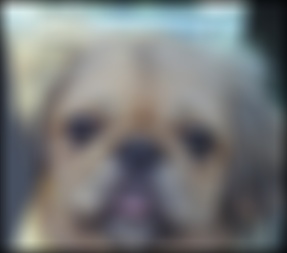
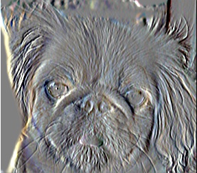
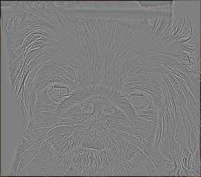
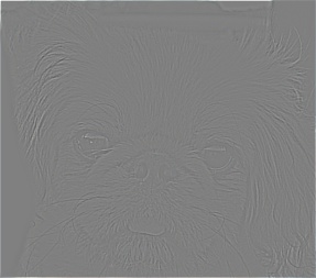
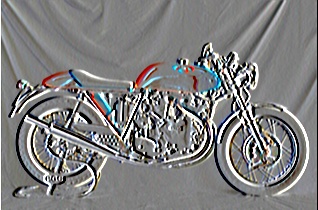
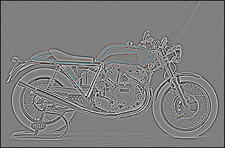
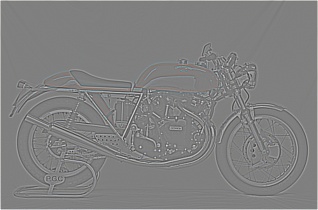
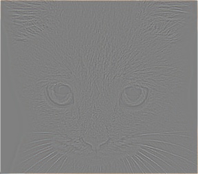
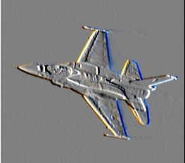
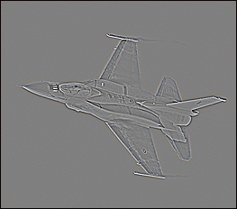
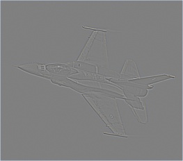
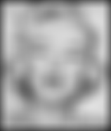
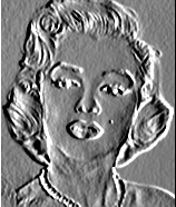
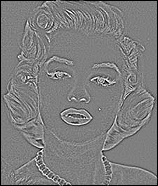
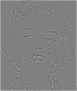
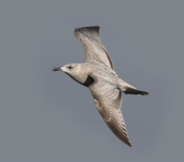
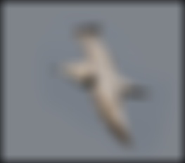
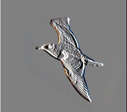
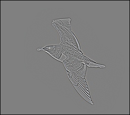
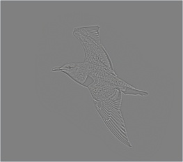
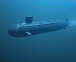
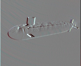
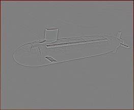
Image Filtering Results using various filters
using variant 1
| Identity Filter | Box Filter | Gaussian Filter | Sobel Filter | Discrete Laplacian Filter | High Pass Filter |

|

|
|
|
|
|
|
|

|
|
|
|

|
|

|
|
|
|
|
|
|
|
|
|
|
|
|
|
|
|

|

|

|
|
|
|

|

|
|
|
|
|
|

|
|
|
|

|
|

|
|
|
|
|

|
|

|
|
|
|
The above results are obtained using the algorithm as mentioned in variant 1.
Comparison of Image Filtering Results
| Using variant 1 | Using variant 2 | Using variant 3 | Using variant 4* |
|
|

|

|

|
| time taken: 2.3sec | time taken: 3.6sec | time taken: 1.9sec | time taken: 2.6sec |
|
|

|

|
|
| time taken: 1.8sec | time taken: 2.8sec | time taken: 1.7sec | time taken: 2.1sec |
|
|
|

|

|
| time taken: 2.2sec | time taken: 3.3sec | time taken: 1.7sec | time taken: 2.4sec |
|
|

|

|

|
| time taken: 1.5sec | time taken: 2.5sec | time taken: 1.3sec | time taken: 2.9sec |
|
|

|
|

|
| time taken: 0.8sec | time taken: 1.3sec | time taken: 0.6sec | time taken: 1.0sec |
|
|

|

|

|
| time taken: 1.9sec | time taken: 3.2sec | time taken: 1.6sec | time taken: 2.3sec |
|
|
|

|

|
| time taken: 1.6sec | time taken: 2.7sec | time taken: 1.5sec | time taken: 2.0sec |
|
|

|
|
|
| time taken: 1.8sec | time taken: 3.0sec | time taken: 1.5sec | time taken: 2.2sec |
|
|

|
|

|
| time taken: 1.6sec | time taken: 2.7sec | time taken: 1.4sec | time taken: 2.0sec |
|
|

|

|
|
| time taken: 0.8sec | time taken: 1.3sec | time taken: 0.6sec | time taken: 1.0sec |
The table above compares the results obtained using a gaussian filter with each of the above variants. Specifically, gaussian filter has been used since the images clearly have some difference along the boundaries.
*- time excludes the time taken to start and shut down a parallel pool.
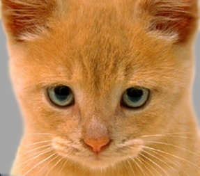
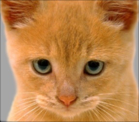
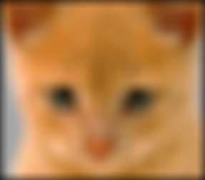
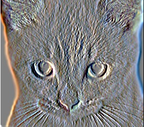
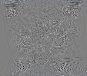
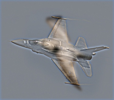
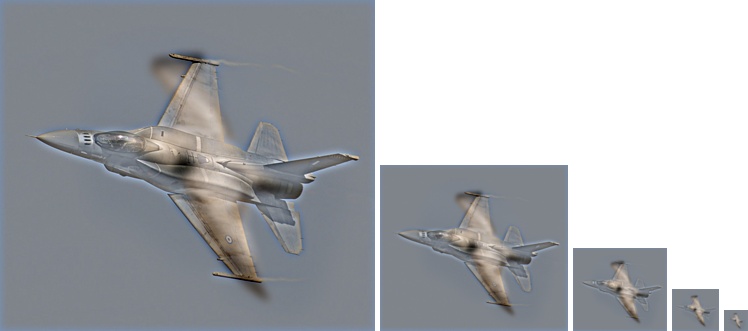
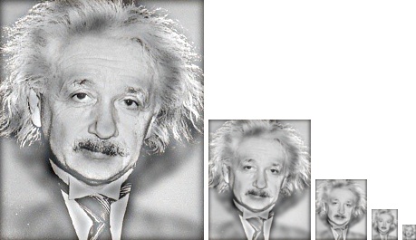
Hybrid Images
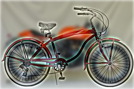
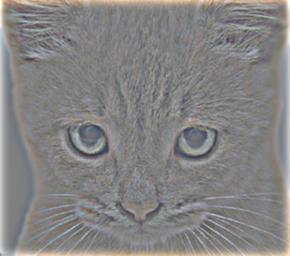
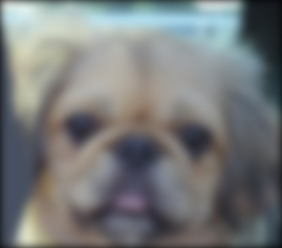
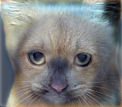
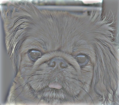
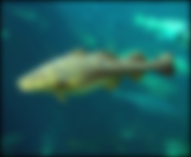
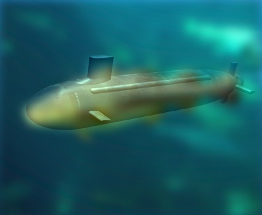
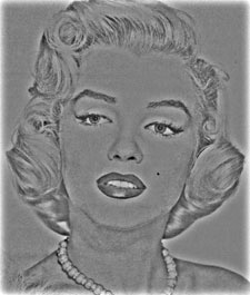
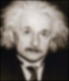
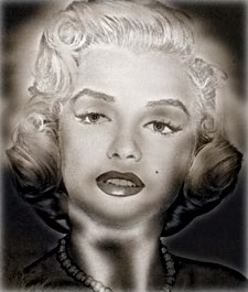
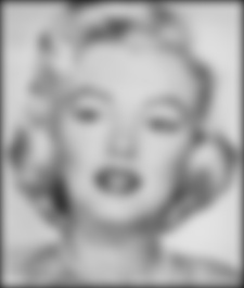
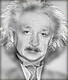
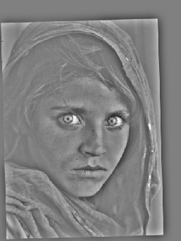
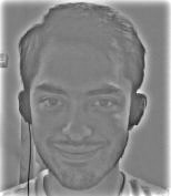
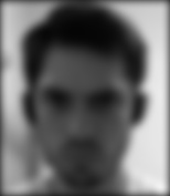
The algorithm to construct hybrid images is present in the file 'proj1.m'. One important change (in 'proj11.m' only) is that the gaussian filter is implemented as a one dimensional filter to reduce the time for computation of the fitered image. The input image is filtered twice once with the gaussian filter and the result with the transpose of the filter to obtain the final filtered image. The low frequencies image is obtained using a gaussian filter on image1 and the high frequencies image of image2 is obtained by subtracting the low frequencies image from the original input image2.The Hybrid image is constructed by adding these two filtered images.
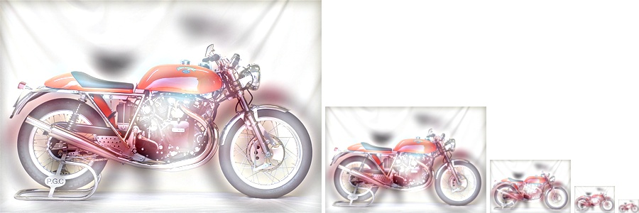
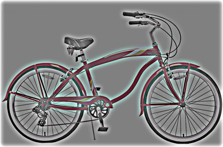
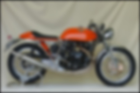
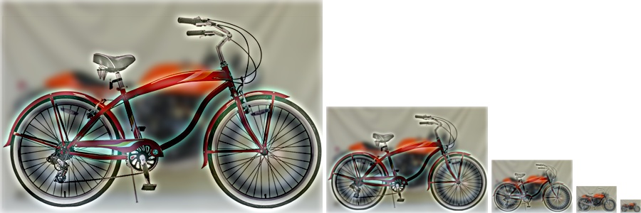
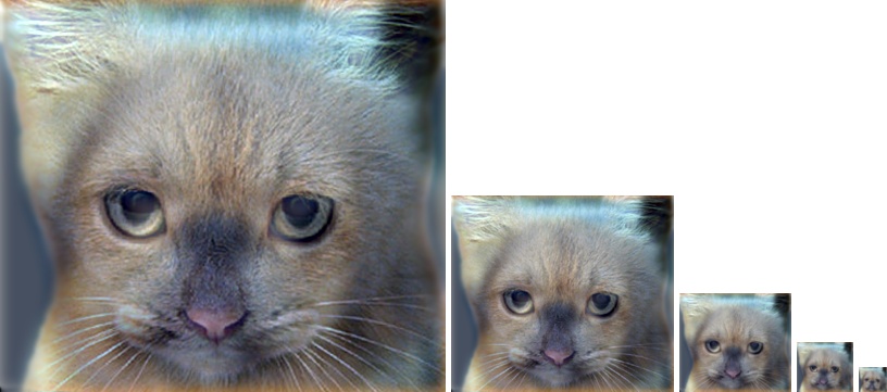
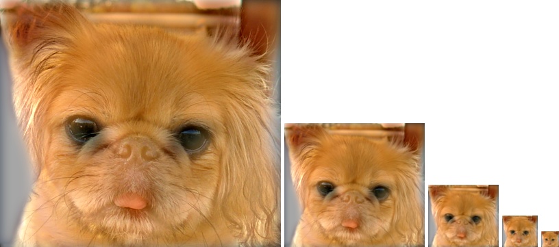
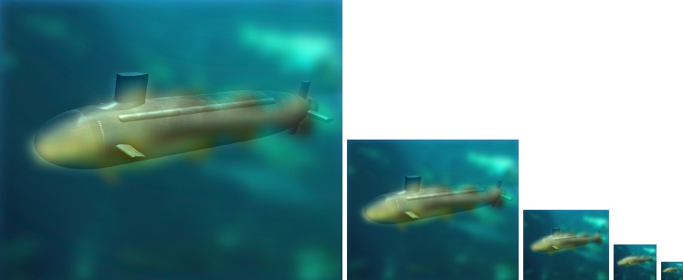
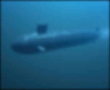
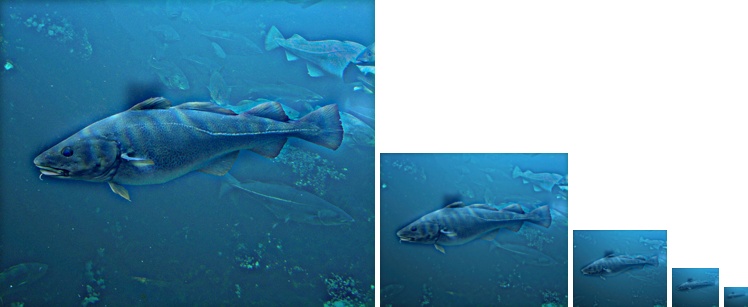
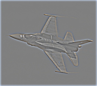
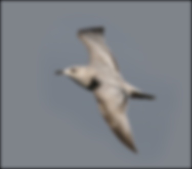
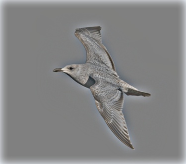
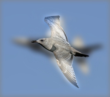
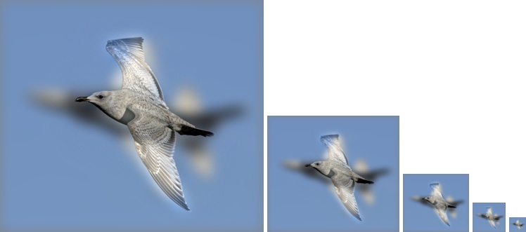
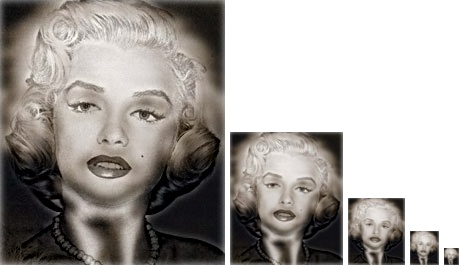
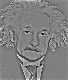
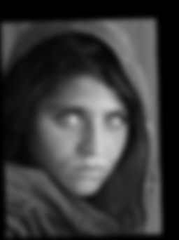
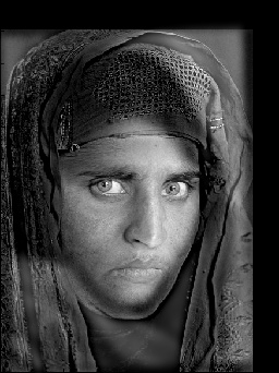
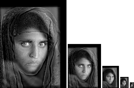
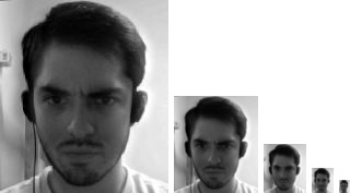
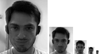
Clearly, the hybrid images would change depending on the image chosen for image1 (low frequencies) and the image chosen for image2(high frequencies). All the corresponding pairs and their results have been present below.
| High Frequencies | Low Frequencies | Hybrid Image | Hybrid Image scales | |
|
|
|
|
|
|
|
|
|
|
|
|
|
|
|
|

|

|
|
|
|
|
|
|
|
|
|

|
|
|
|
|
|
|
|
|

|
|
|
|
|
|
|
|
|
|
|
|
|
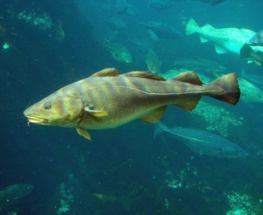
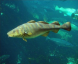
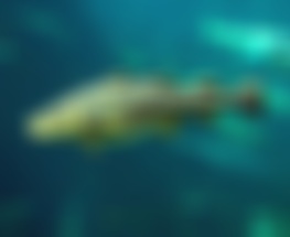
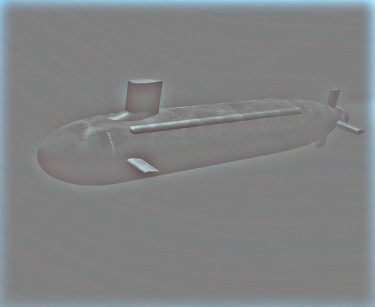
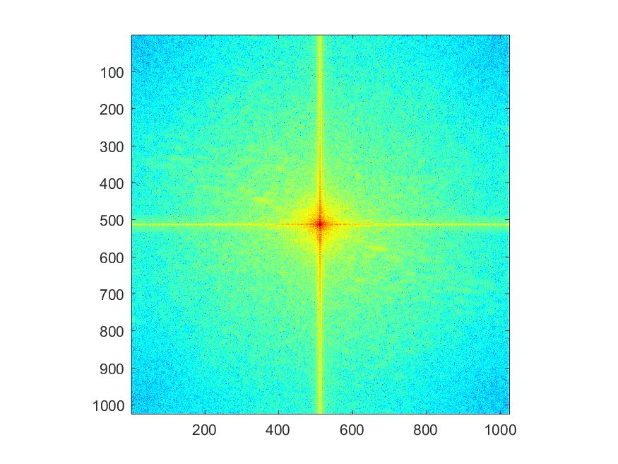
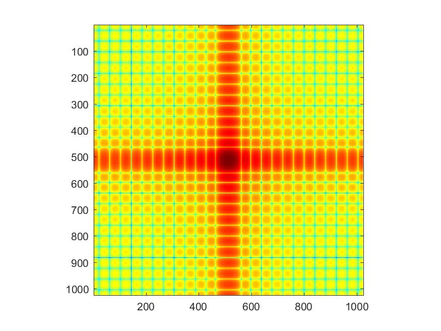
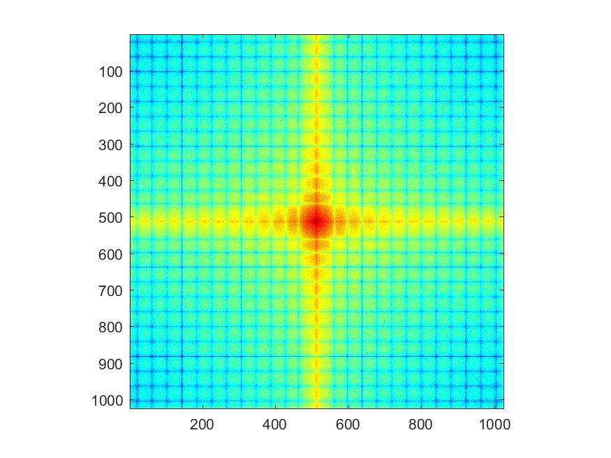
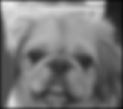
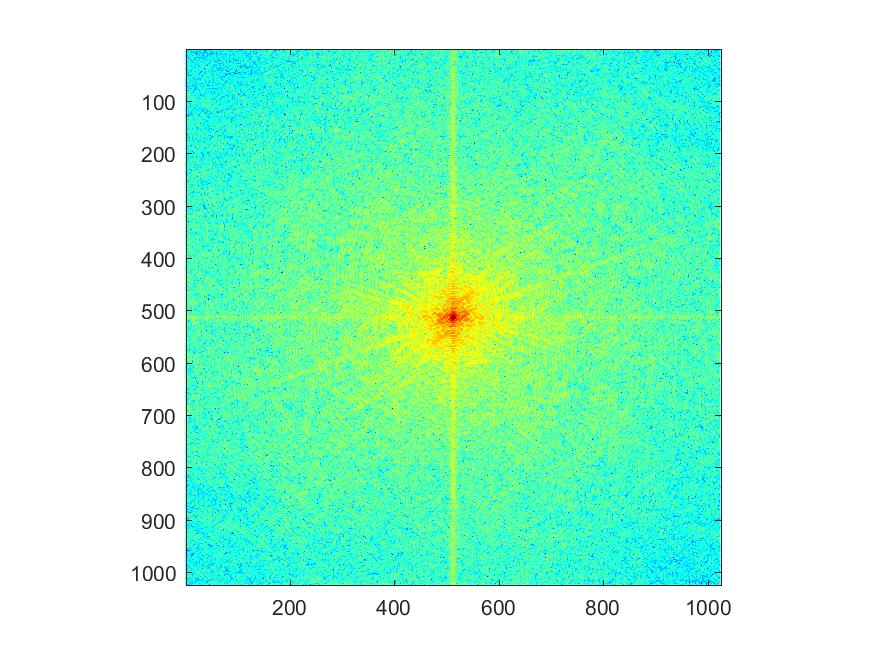
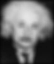
Image Filtering in the frequency domain
I have also implemented the image filtering of the grayscale image of the input image in the frequency domain using a gaussian filter in 'myfilter_freq.m' file. The code uses inbuilt function in matlab on fourier transform and inverse fourier transform.
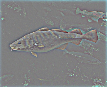
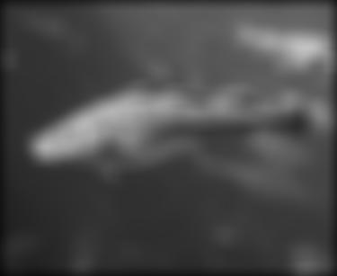
im = double(imread('../data/fish.bmp'))/255;
im = rgb2gray(im); % “im” should be a gray-scale floating point image
[imh, imw] = size(im);
hs = 12; % filter half-size
fil = fspecial('gaussian', hs*2+1, 10);
fftsize = 1024; % should be order of 2 (for speed) and include padding
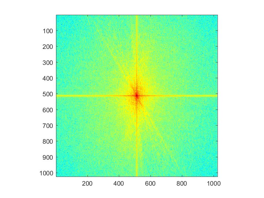
im_fft = fft2(im, fftsize, fftsize); % 1) fft im with padding
figure(1), imagesc(log(abs(fftshift(im_fft)))), axis image, colormap jet; saveas(figure(1),'image_fft.jpg');
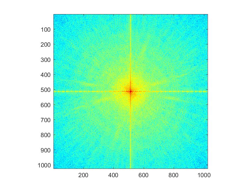
fil_fft = fft2(fil, fftsize, fftsize); % 2) fft fil, pad to same size as
figure(2), imagesc(log(abs(fftshift(fil_fft)))), axis image, colormap jet; saveas(figure(2),'filter_fft.jpg');
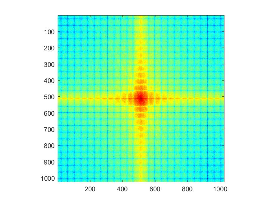
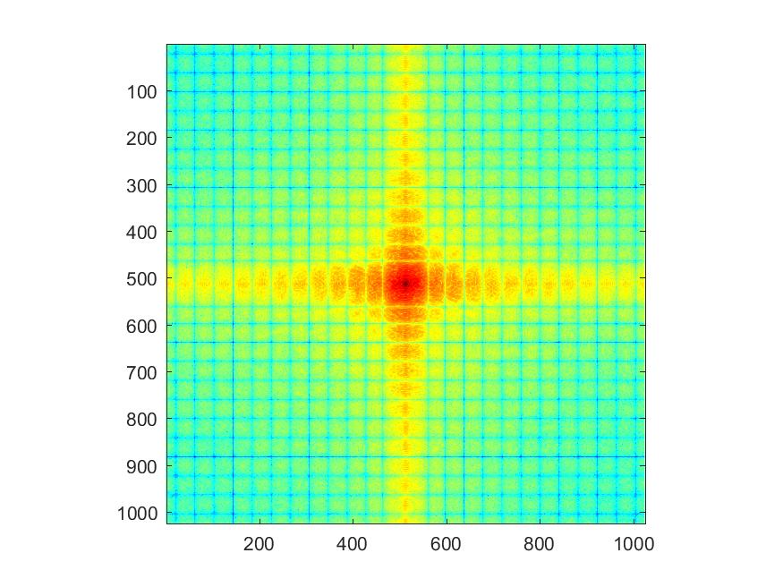
im_fil_fft = im_fft .* fil_fft; % 3) multiply fft images
figure(3), imagesc(log(abs(fftshift(im_fil_fft)))), axis image, colormap jet; saveas(figure(3),'image_filter_fft.jpg');
im_fil = ifft2(im_fil_fft); % 4) inverse fft2
im_fil = im_fil(1+hs:size(im,1)+hs, 1+hs:size(im, 2)+hs); % 5) remove padding
figure(4), imshow(im_fil); imwrite(im_fil, 'filtered_image.jpg');
output=im_fil;
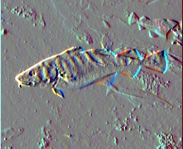
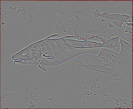
| Input Image | FFT of Image | FFT of filter | FFT of Image.*filter | Filtered image | |
| Dog |
|
|
|
|
|
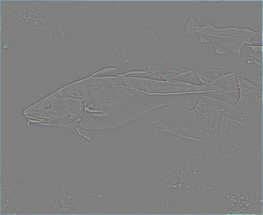
| Fish |
|

|
|
|
|
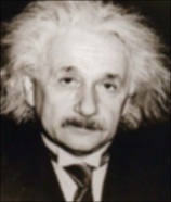
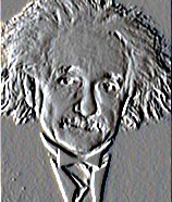
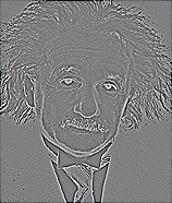
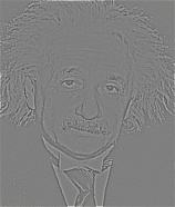
| Einstein |
|

|
|
|
|
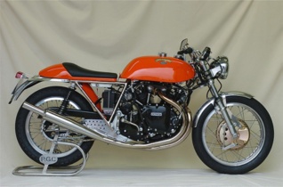
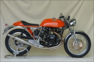
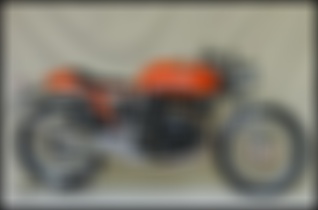
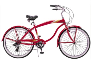
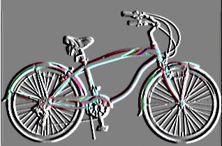
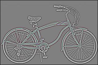
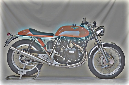
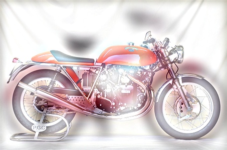
| Bicycle |
|

|

|
|
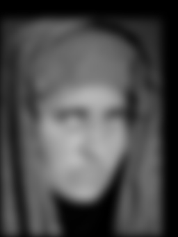
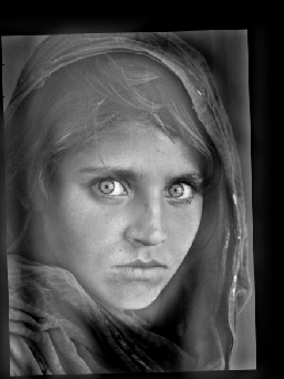
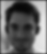
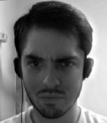
Additional examples for Hybrid Images
The following examples which are given below are also used for the generation of hybrid images. The results are presented below. The same algorithm as mentioned above has been used for the hybrid images.
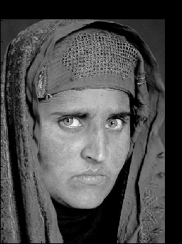
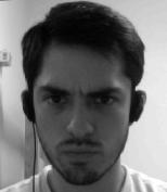
| Young Girl | Woman | Happy | Angry | |

|
|

|
|
For the above examples, we used a guassian filter with an appropriate cuttoff frequency and then the hybrid images are generated as shown below.
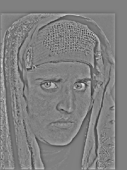
| High Frequencies | Low Frequencies | Hybrid Image | Hybrid Image scales | |
|
|
|
|
|
|
|
|

|
|

|
|
|
|
|
|
|

|
|
All the work that has been implemented for the project has been presented and discussed above. Feel free to contact me for further queries.
Contact details:
Murali Raghu Babu Balusu
GaTech id: 903241955
Email: b.murali@gatech.edu
Phone: (470)-338-1473
Thank you!