Project 1: Image Filtering and Hybrid Images
Author: Mitchell Manguno (mmanguno3)
Table of Contents
Synopsis
For this project, an image filtering function was written and then used to produce "hybrid images" of pairs of images. Hybrid images are defined here in a paper by Oliva, Torralba, and Schyns. Essentially, two images are taken into consideration. One is filtered such that all that remains are the low frequency componenets of the image; the other, only high frequency components remain. When blended, this images appear differently at varying viewing distances.
I will now explain in detail the image filtering function, and present the result of using this function to create hybrid images.
Image Filtering
The algorithm used for the function closely follows the classical definition of filtering: given a image f and a filter g, the output image h is defined as:
h[m, n] = Σk, l g[k, l] f[m+k, n+l]
Each element of h is the inner product of the filter and the region upon which the filter is situated. With this consideration, the function can be made a bit simpler to reason about, and can utilize some of MATLAB's functions (which are faster to run than using for-loops, due to their implementation in FORTRAN).
// Calculate the appropriate amount to pad
extra_rows = floor(num_rows(filter) / 2);
extra_cols = floor(num_cols(filter) / 2);

// Pad the image symmetrically by the extra rows and columns
padded = pad_image_symmetrically(image, extra_rows, extra_cols;

for m from 1 ... num_rows(image)
    for n from 1 ... num_cols(image)
        // Get the region of the padded image to filter
        region = padded[m ... num_rows(filter) + m, n ... num_cols(filter) + n]
        // The value of the output at [m, n] is the inner product of the
        // filter and the region
        output[m, n] = filter · region
The above code was implemented in MATLAB, and run to produce the results seen below.
It's worth noting two things about the design of this algorithm:
- It uses as few for-loops as it reasonably can, without butchering readability. This is because MATLAB's language-level constructs are slow, but the matrix operations that are in its standard library are very fast (by virtue of their implementation in FORTRAN).
- The image is being padded symmetrically, rather than with zeros or in some other manner. This is done to preserve nearby pixel information without introducing undue noise in a sensible way.
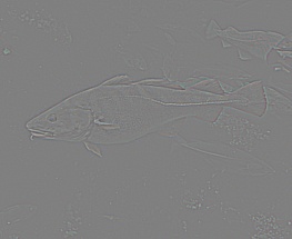
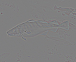
Here are some of the results of the filtering algorithm on a picture, with different filters applied.
 |
 |
 |
| fig. 1 identity filter | fig. 2 blur filter | fig. 3 large blur filter |
 |
 |
 |
| fig. 4 high pass filter | fig. 5 laplacian filter | fig. 6 sobel filter |
As you can see, the filters appear to work well on the images, and no strange discolorations occur around the edges of the images since a symmetrical padding strategy was used.
Hybrid Images
With the above algorithm, five hybrid images were produced, drawn from ten total images. The pairings were images of:
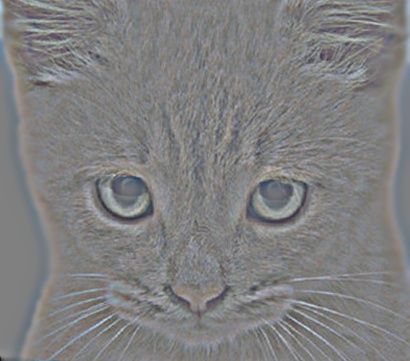
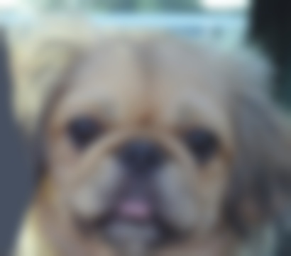
- a cat and a dog;
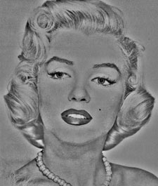
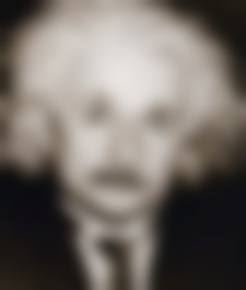
- Albert Einstein and Marilyn Monroe;
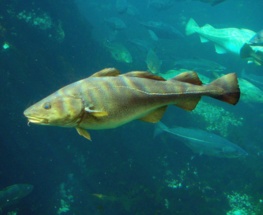
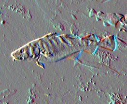
- a fish and a submarine;
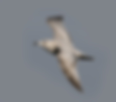
- a bird and a fighter jet; and,
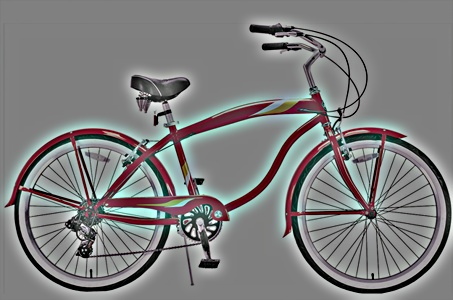
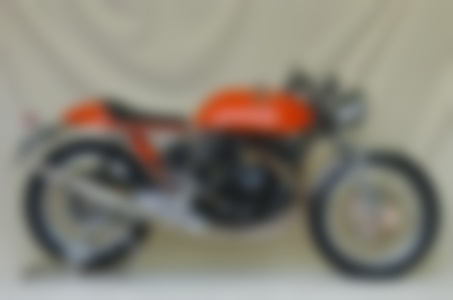
- a motorcycle and a bicycle
From the gallery below, it is clear to see that the hybird images do indeed appear differently depending on viewing distance.
Gallery
Cat and Dog
 |
 |
 |
| fig. 7 high frequency image | fig. 8 low frequency image | fig. 9 hybrid image |
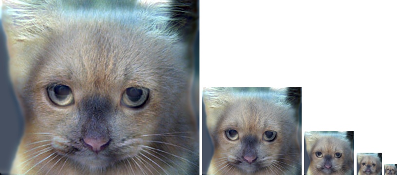 |
| fig. 10 hybrid image scaled sequence |
Einstein and Monroe
 |
 |
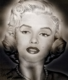 |
| fig. 11 high frequency image | fig. 12 low frequency image | fig. 13 hybrid image |
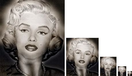 |
| fig. 14 hybrid image scaled sequence |
Fish and Submarine
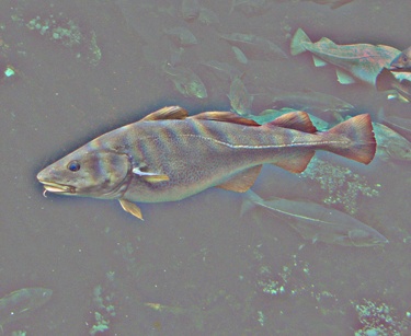 |
 |
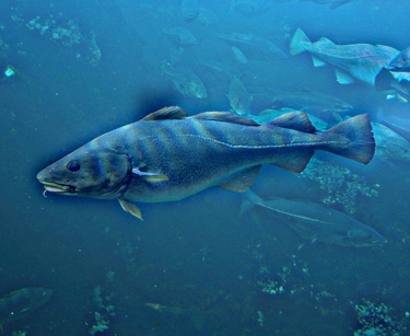 |
| fig. 15 high frequency image | fig. 16 low frequency image | fig. 17 hybrid image |
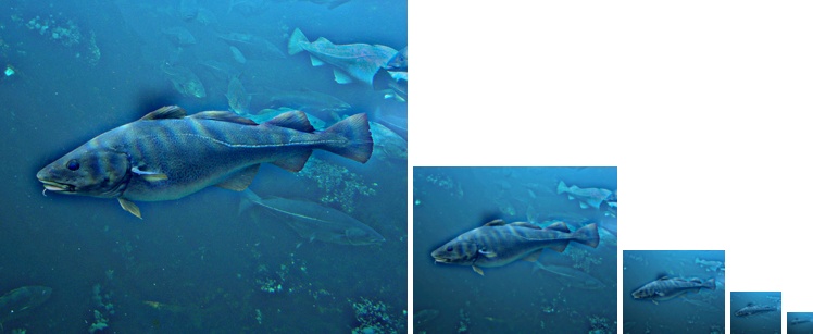 |
| fig. 18 hybrid image scaled sequence |
Bird and Plane
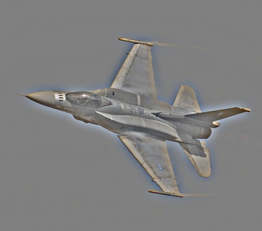 |
 |
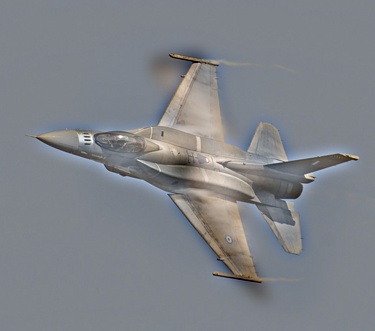 |
| fig. 19 high frequency image | fig. 20 low frequency image | fig. 21 hybrid image |
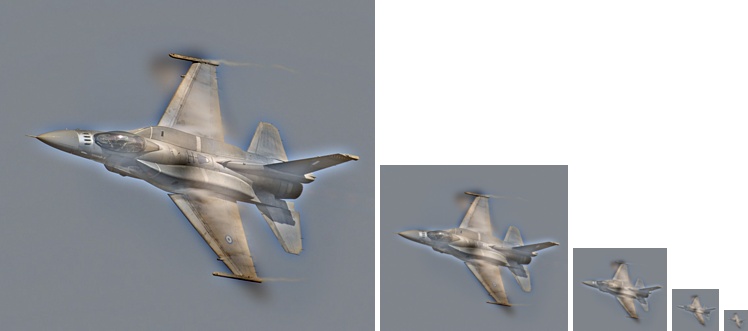 |
| fig. 22 hybrid image scaled sequence |
Motorcycle and Bicycle
 |
 |
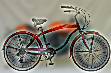 |
| fig. 23 high frequency image | fig. 24 low frequency image | fig. 25 hybrid image |
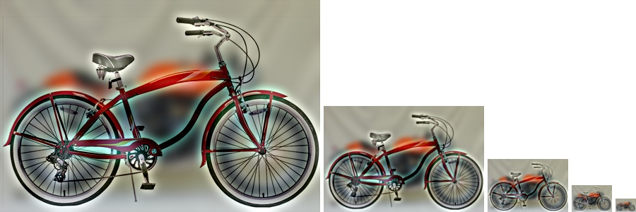 |
| fig. 26 hybrid image scaled sequence |