Project 1

Image Filtering

Image filtering (or convolution) in computer vision is a technique to add, enhance or remove features by applying a filter to an image. It is an image processing technique which has many applications ranging from enhancing the image for noise removal, sharpening, deblurring, etc. MATLAB provides a function knows as imfilter (image, filter) which performs convolution on an image using a filter.

Comparison of MATLAB's **imfilter** and **my_imfilter**
	imfilter	my_imfilter
Original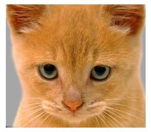
Identity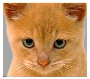
Small Blur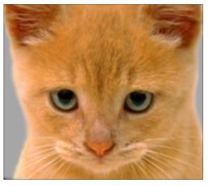
Large Blur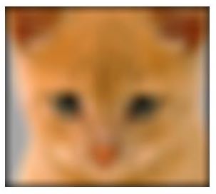
Oriented (Sobel)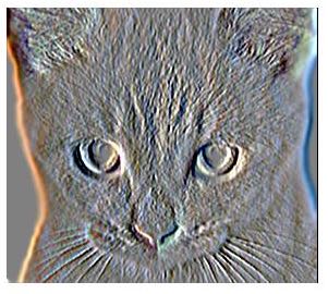
High Pass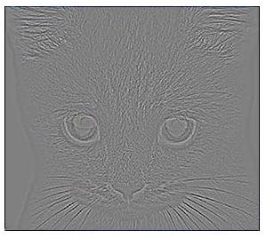
High Pass (alternate)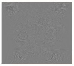

The my_imfilter function is implemented using the following steps:

Handle greyscale and color images
Reading all 3 dimensions of the image size ensures that we capture data regarding the type of image in the 3rd argument. In the following piece of code image_scale is used to store the color type (the code can also handle any other value of image_scale).


%Read image dimensions
[image_height, image_width, image_scale] = size(image);

% image_scale == 1 implies GreyScale
% image_scale == 3 implies Color

Handle filters of different sizes (odd-numbered)
By padding the image based on a filter size, we can ensure that we can,
- Apply filters of any size (that have odd numbered dimensions).
- Not lose any information from the original image,.ie., we can use all pixels for filtering.
- Perform convolution without any conflict in matrix operations.
```
padsize = [(filter_height-1)/2,(filter_width-1)/2];
```
Reflect the input image using padarray
While padding, using mirror reflection along the edges provides better results than zero padding. From the comparison table above we see that for my_imfilter for a "large blur", the edges are uniform and smooth whereas for imfilter the edges are dark.
```
padded_image = padarray(image, padsize, 'symmetric');
```

Filter the image
By looping over the image_height, image_width, and image_scale, we can apply the filter to the image by performing an element wise dot product over filter-shaped boxes in the image.


% Find dimensions
[padded_image_height, padded_image_width, padded_scale] = size(padded_image);

% Convolution
for i= 1:image_height
    for j= 1:image_width
       for k=1:image_scale
           padded_image_copy(i+padsize(1),j+padsize(2),k) 
           = sum(sum(padded_image(i:i+filter_height-1,j:j+filter_width-1,k).*filter));
        end
    end
end

% Crop the output to original size and return
% output = padded_image_copy(1+padsize(1):padded_image_height-padsize(1),
%				1+padsize(2):padded_image_width-padsize(2),:);
output = imfilter(image, filter);

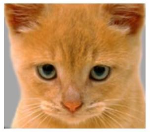
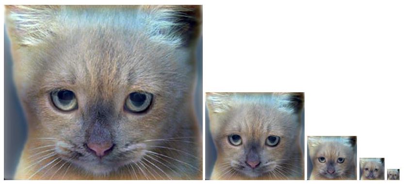
2. Hybrid images

Implementation

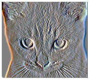
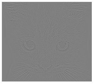
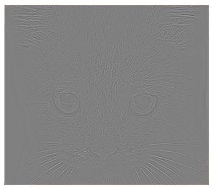
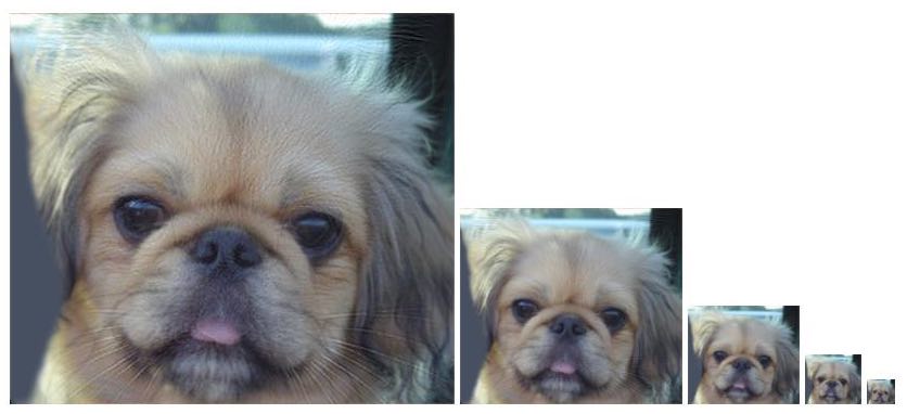
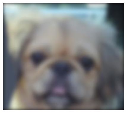
We find the low frequency image of our first image by convolving it with a Gaussian filter of low frequency. We also find the low frequency image of the second image (blur_image) and subtract this from its original to obtain the high frequency image of the second image.
By summing up these two outputs we obtain the hybrid image.


% read images and convert to floating point format
image1 = im2single(imread('../data/dog.bmp'));
image2 = im2single(imread('../data/cat.bmp'));

% set cutoff_frequency and filter
cutoff_frequency = 7;
filter = fspecial('Gaussian', cutoff_frequency*4+1, cutoff_frequency);

% image with low_frequencies
low_frequencies = my_imfilter(image1,filter);

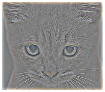
% image with high_frequencies
blur_image = my_imfilter(image2, filter);
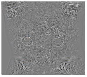
high_frequencies = image2 - blur_image;

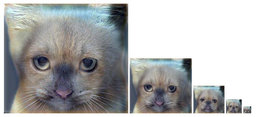
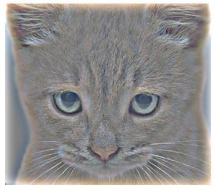
% compute the hybrid_image
hybrid_image = low_frequencies + high_frequencies;

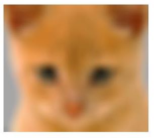
Choosing the right cut-off frequency

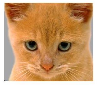
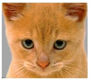
By experimenting with different cut-off frequencies, we get 7 as the ideal frequency for the cat and dog images. The ideal frequency would be the one where the high frequency image is dominant but the low frequency image only acts as noise in the image.

Frequency	Dog	Cat	Hybrid
2
7 (best)
50

Experimenting with new images

Note: No hybrid images have been made using these images before.
By trying out if hybrid images work on similar images, I came across 2 scenarios as given below where the filter created new hybrid images. However, this process involved pre-processing which was done by finding similar images, cropping and reflecting them such that align on top of each other.

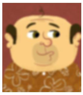
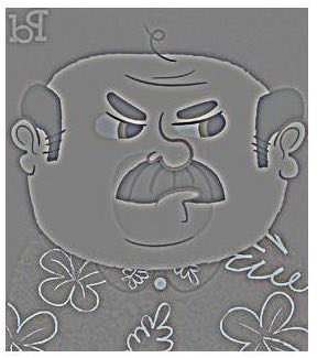
(1) Happy or Angry?

Here, we take the low frequencies of the image with a happy face and the high frequencies of the of the image with a sad image. From a short distance we see an angry man and as we move away from the image we see a happy man.

Happy	Angry	Hybrid

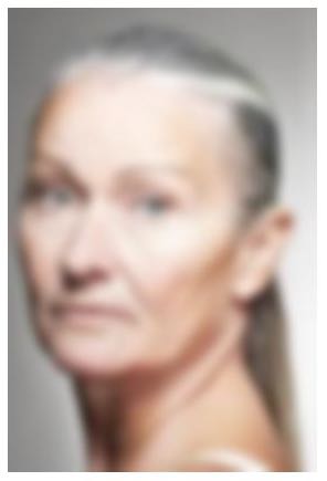
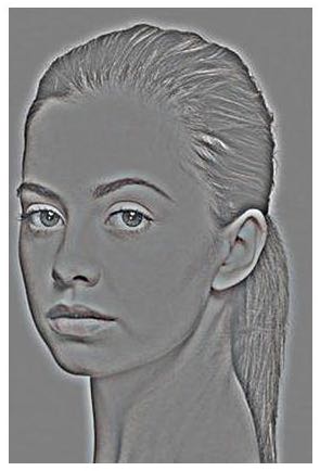
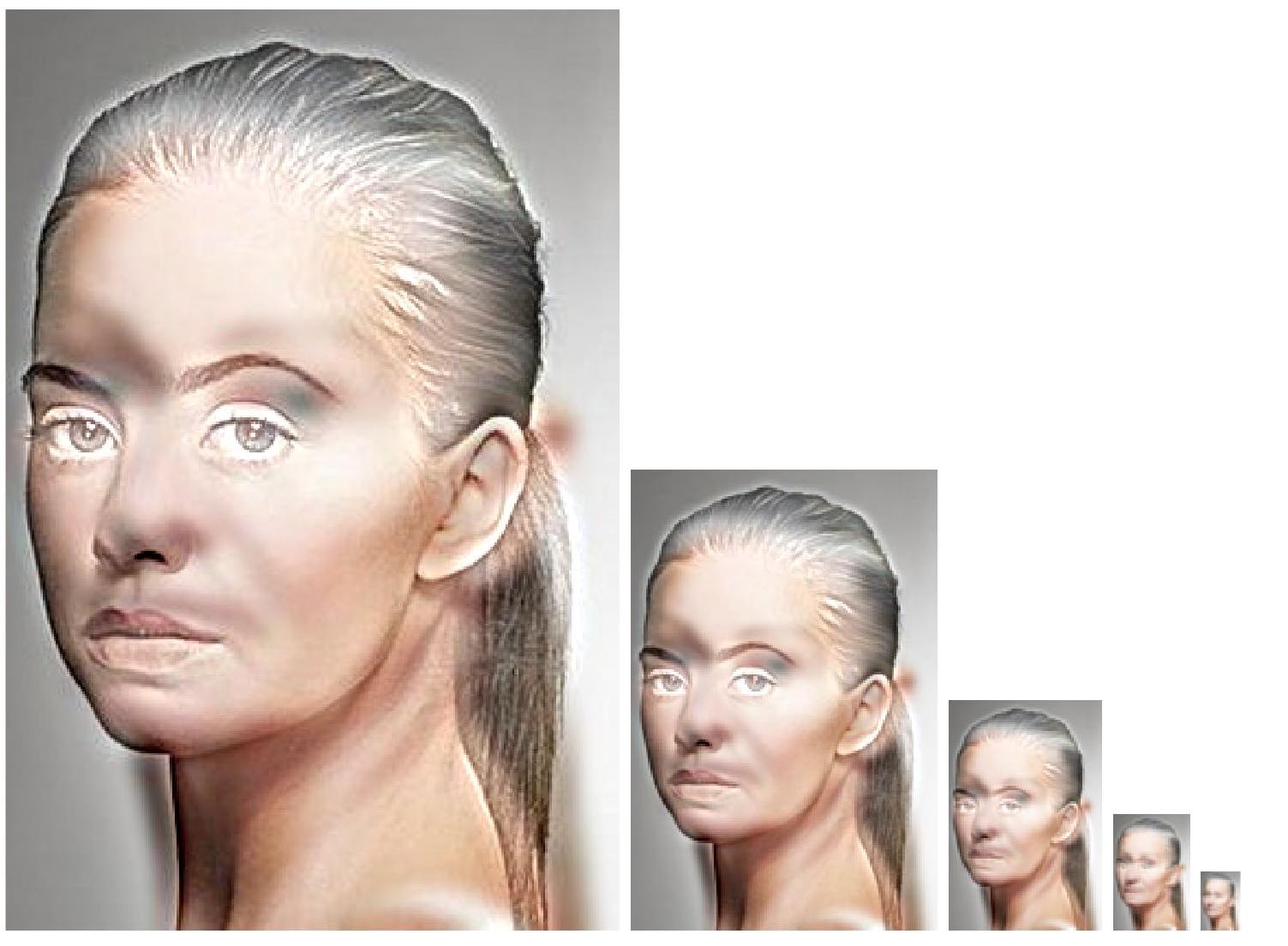
Aging (Time Lapse)

Similarly, we take the low frequencies of the image with an old woman and the high frequencies of the image with a young woman. From a short distance we see a young woman and as we move away from the image we see an old woman.

Old	Young	Hybrid

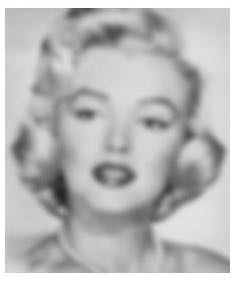
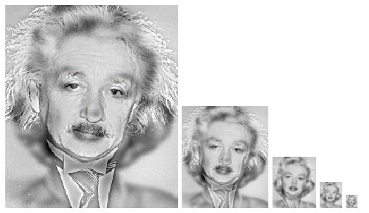
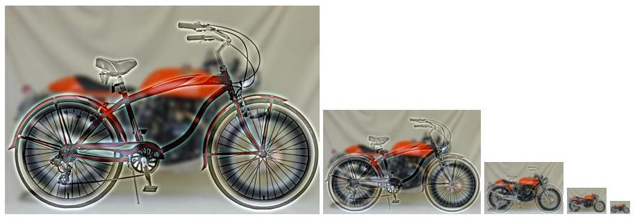
Experimenting with existing images

We can try modifying the cutoff frequencies for different images, and we obtain the following output.

Best Cut-Off Frequency	Image1	Image2	Hybrid
Marilyn - Einstein 4
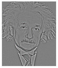Submarine - Fish 3
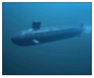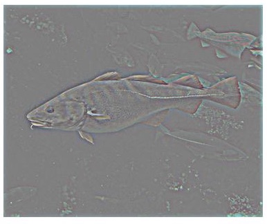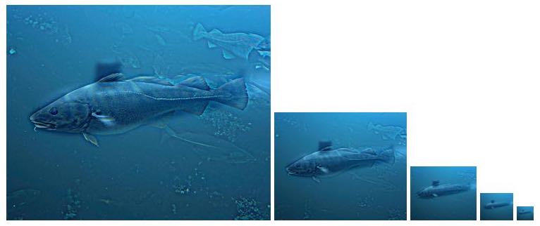Plane - Bird 6
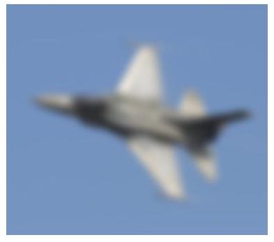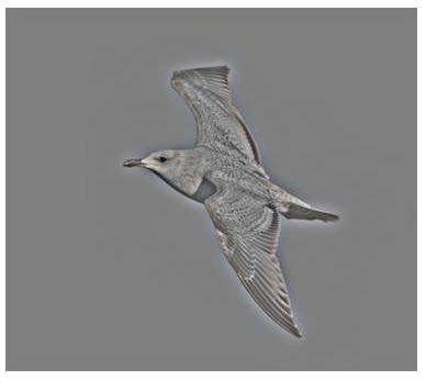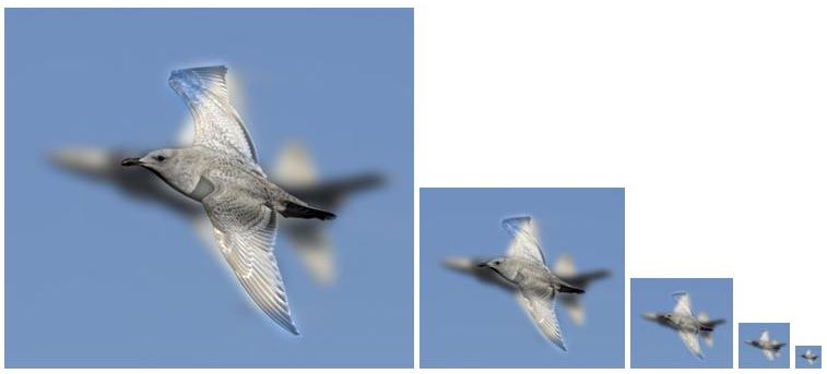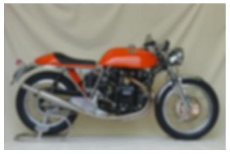
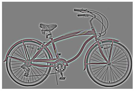
Bike - Cycle 4

We see that we can modify the filter size or the cutoff frequency (or the sigma of the Gaussian) to obtain the right kind of blending required to produce a Hybrid Image.

Meghna Natraj