Project 1: Image Filtering and Hybrid Images
A hybrid image example of a cat and a dog
The main focus of this project is imitating the imfilter() function in MATLAB to perform image filtering in the spatial domain on either a grayscale image or a color image using an arbitrary sized filter (except that it has to be of odd dimensions). Learning from the in-class lecture, I know that the idea is to compute the function of the local neighborhood at each pixel of the image. The local neighborhood depends on the size of the filter. In order to not miss out on computing and filtering the pixel rows and columns along the image borders, I have to pad the input image around its borders. Padding is basically a procedure to add rows and columns of either zeros or reflected pixels around the image borders. Therefore, the first thing I did to the starter code was to ensure my function is able to determine the filter size, which leads to the padding of the input image with the correct number of rows and columns around its outer boundary. The build-in MATLAB function padarray provides us easy way to surround the image with either zeros or reflected pixels along the image boundary. With the input image successfully padded according to the filter size, I could move on to construct the filtering algorithm, or simply put, to compute the filtered intensity value of each pixel location on the original image. Since the filter is a matrix of arbitrary odd dimensions, I decided to separate the 3-dimensional (3-D) image, which could be a color image, into its separate Red(R) matrix, Green(G) matrix, and Blue(B) 2-D matrix. I then created a virtual 2-D rectangle that is of the same size of the filter and superimpose it on say the R matrix at its top left corner. The virtual 2-D rectangle is a matrix that contains the pixel values of the image on which it is being superimposed. By computing the dot product between the virtual 2-D rectangle and the filter, I was able to obtain the filtered pixel value of a specific pixel location. The virtual rectangle is circulated through every row and column of each of the R, G, and B matrices of the padded input image using three For-loops until every pixel location of the original image contains a filtered pixel value. The rows and columns around the image borders that have been padded with trivial values are removed so that the output image has the same resolution as the input image. The R, G, and B matrices are also concatenated into one single 3-D output image file.
Extra Work
I also scripted my own code for padding the input image with reflected pixels along the image borders, without using the build-in function padarray. Once the number of rows and columns required for padding is computed based on the filter size, I used a For-loop to pad the top and bottom of the input image. I then proceeded to use another For-loop to pad the left and right columns of the input image with reflected pixels along the vertical borders. The algorithm is looped through each of the R, G, and B matrices of the input image. This self-developed code has been proven to work well as it leads to exactly same resultant image and takes similar amount of computation time as when padarray is used, at least for the given filters.
%% self-developed code for padding reflection values
sizeF = size(filter);
rowF = sizeF(1);
colF = sizeF(2);
t = image;
for j = 1:1:3
t1 = t(:, :, j);

        sizet1 = size(t1);
        rowt1 = sizet1(1);
        colt1 = sizet1(2);
        t1_new = t1;
        rowneeded = (rowF-1)/2;
        if rowneeded >0
            for i=1:rowneeded
                TopR(i,:) = t1(i,:);
                t1_new = vertcat(TopR(i,:),t1_new);
                BotR(i,:) = t1(rowt1+1-i,:);
                t1_new = vertcat(t1_new,BotR(i,:));
            end
        end
        t1_new2 = t1_new;
        colneeded = (colF-1)/2;
        if colneeded >0
            for i=1:colneeded
                LeftC(:,i) = t1_new(:,i);
                t1_new2 = horzcat(LeftC(:,i),t1_new2);
                RightC(:,i) = t1_new(:,colt1+1-i);
                t1_new2 = horzcat(t1_new2,RightC(:,i));
            end
        end
        if j == 1
        R1 = t1_new2;
        else if j == 2
        G1 = t1_new2;
        else if j == 3
        B1 = t1_new2;
            end
            end
        end
end
%% ImageNew1 is the image with padded reflections around its edges
ImageNew1 = cat(3, R1, G1, B1);
Results
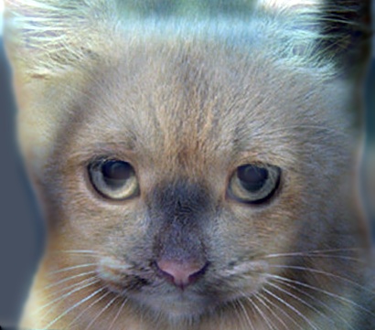
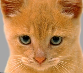
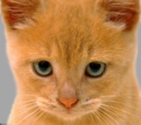
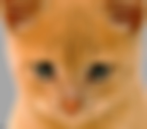
Using the low pass Gaussian filter and the my_imfilter function, a low frequency image can be generated. By subtracting the low frequency image from the original input image, a high frequency image can then be generated. The hybrid images as shown in the table below are created by adding the low frequency image and the high frequency image. As we can see from the images which have been progressively downsampled, the high frequency image always dominates our perception when we view the largest image (close image) while the low frequency image dominates our perception when we view the smallest image (far image). Five pairs of images are provided and tested while the cutoff frequency is tuned specifically for each pair of images. The cutoff frequency is tuned by adjusting the standard deviation, in pixels, of the Gausian filter (low pass filter) to provide the best visual results.Testing different filters on the cat image:
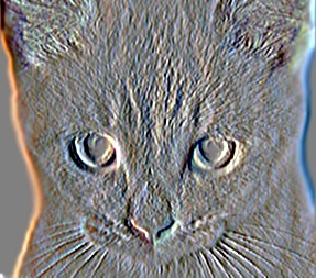
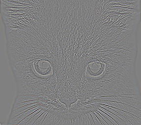
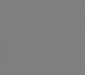
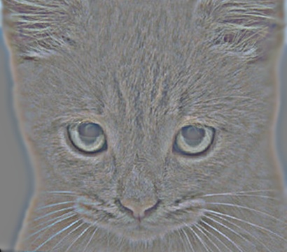
Identity image Small blur Large blur Sobel filter
Discrete Laplacian image High pass "filter"
|
Hybrid Images:

Low frequency dog High frequency cat
|
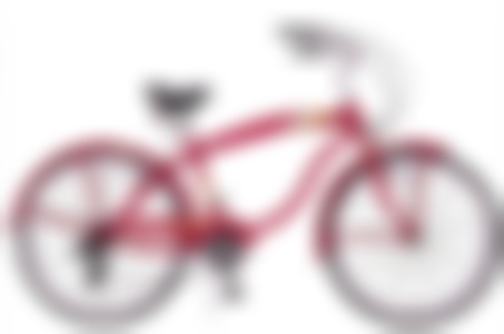
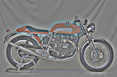
Low frequency bicycle High frequency motorcycle
|
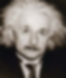
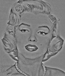
Low frequency Einstein High frequency Marilyn
|
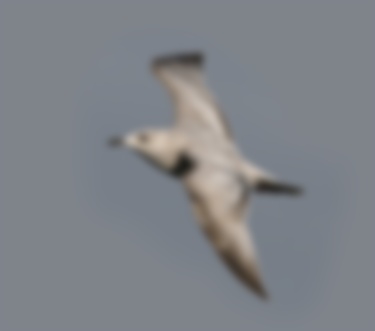
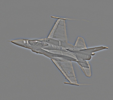
Low frequency bird High frequency plane
|
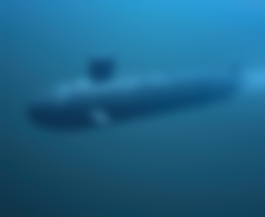
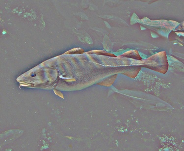
Low frequency submarine High frequency fish
|
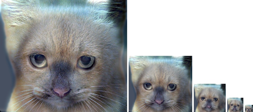 cutoff frequency = 7
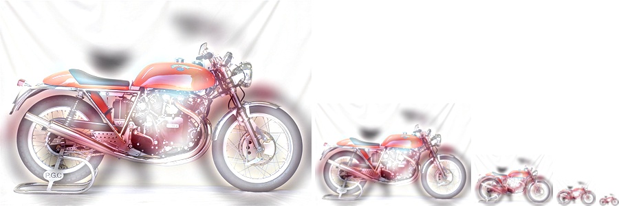 cutoff frequency = 9
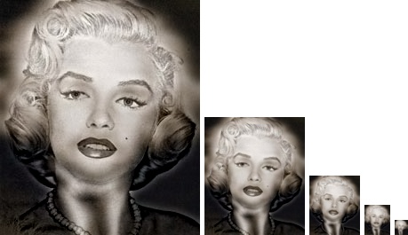 cutoff frequency = 5
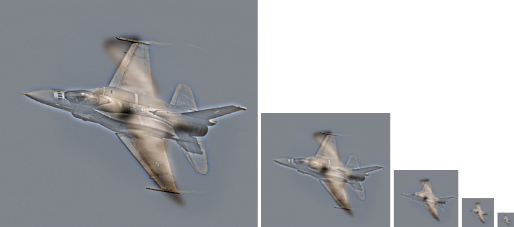 cutoff frequency = 4
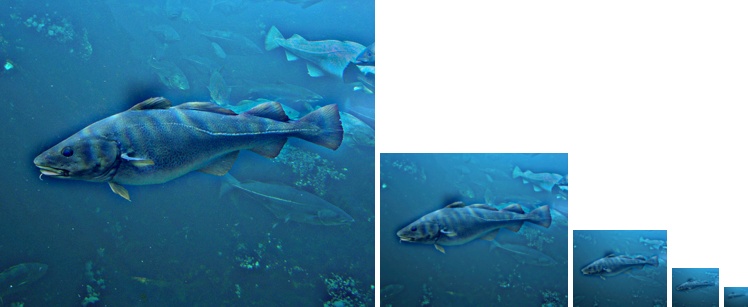 cutoff frequency = 7