CS 6476 Project 1: Image Filtering and Hybrid Images
Image Source: Jain, R., Kasturi, R., Schunck, B. Machine Vision.
In this project, we explore an image processing technique known as filtering to modify and enhance pictures. Filtering consists of neighborhood operations that can be used to sharpen details, blur edges, remove random noise, and accentuate edges in an image. When a 2D-image is filtered, the process involves moving a 2D sliding window, called a kernel, across the image and computing the weighted sum of input pixel values with corresponding kernel values to obtain the filtered image's output pixel value. For simplicity, we limit the scope of this discussion by only considering linear filters, which obey the
- Superposition principle
- Shift-invariance principle
For the first part of the project, we are tasked with implementing my_imfilter(), an identical version of MATLAB's imfilter() function. my_imfilter() accepts two arguments:
-
image, a matrix representing an image, and -
filter, a kernel with odd dimensions that will be used to perform the filtering operation on the image.
After implementing my_imfilter(), the second part of the project is the creation of hybrid images by combining a low-pass filtered image (blurred) with a high-pass filtered image (sharpened). When the hybrid image is viewed up close, the eyes perceive primarily the high spatial frequencies. When viewed from a distance, these high spatial frequencies components in the image disappear, and our eyes are only able to perceive the low spatial frequencies.
Image Filtering
Image filtering is governed by the following equation:
where
g(i, j) = the value of the output pixel at image point (i, j)
f(i, j) = the input pixel value at point (i, j)
h(k, l) = the value at coordinate (k, l) of the kernel h.
Method
In order to construct the filtered image, we first center an kxl kernel h, where k and l are odd, with a pixel (i, j) in the input image; then, we obtain the output pixel value at (i, j) by computing the element-wise dot product between the kxl kernel and the (k,l)-sized neighborhood surrounding the image at that point (i,j).
To address the problem of the kernel window extending past the original image boundaries when filtering border pixels, the input image is padded with 0 pixels along the edges so that the kernel window aligns nicely at those edges. One downside of this approach is that the filtered image appears darker around the borders, which may be bothersome when creating the hybrid images.
my_imfilter() Implementation
function output = my_imfilter(image, filter)
output = imy_imfilter(image, filter, 0);
end

% padtype - takes values 0, 'circular', 'replicate', and 'symmetric'
function ioutput = imy_imfilter(image, filter, padtype)
    [rows, cols, dims] = size(image);
    [m, n] = size(filter); % The kernel is assumed to be odd mxn matrix.
    ioutput = zeros([rows cols dims]);

    % Deals with the issue of the kernel window being out of bounds at the edges.
    % Pads the sides of the image with 0-valued pixels.
    padded_img = padarray(image, floor([m n] ./ 2), padtype);
    convolve_neighborhood = @(region, kernel) sum(sum(region .* kernel));

    % Filter the image by centering the kernel window at every pixel.
    for d=1:dims
        for r=1:rows
            for c=1:cols
                ioutput(r,c,d) = convolve_neighborhood(...
                padded_img(r:r+m-1, c:c+n-1, d), filter);
            end
        end
    end
end
Results
| Identity Image | Original, unfiltered image. | |
| Blur Image | Output image produced by a 3x3 box filter. | |
| Large Blur Image | Output image after blurring with a 25x1 Gaussian filter (σ=10) along horizontal and vertical directions. | |
| High Pass Image | Output image after convolving input with (1-B), where B is the 3x3 box filter. | |
| Sobel Image | Output image displaying prominent vertical edges from the original image. | |
| Laplacian Image | Output image after applying the positive Laplacian operator ([0 1 0; 1 -4 1; 0 1 0]) to the original image. |
Hybrid Images
Method
As mentioned in the Hybrid Images paper, the process of creating a hybrid image from two separate images involves
- Filtering the image to be visible from a distance (I1) with a low pass filter (i.e. Gaussian kernel G1).
- Filtering the image that is visible from up close (I2) with a high pass filter (i.e. 1-G2, where G2 is Gaussian kernel).
- Once these two steps are finished, we simply add the two filtered images together to produce the hybrid image.
hybrid_image = low_frequencies + high_frequencies;
low_frequencies = my_imfilter(image1, filter);high_frequencies = image2 - my_imfilter(image2, filter);The parameter
cutoff_frequency specifies the standard deviation σ for both Gaussian kernels G1 and G2 and must be tuned to produce the appropriate hybrid image. The code provided in proj1.m uses a single cutoff_frequency for both G1 and G2. However, the Hybrid Images paper recommends selecting a separate cutoff_frequency for each filter that corresponds to the frequency when the amplitude gain of the filter is 1/2.
Results: Image Pairs
| Image 1 | Image 2 | Low Frequencies | High Frequencies | Hybrid Image | Cutoff Frequency | |
|---|---|---|---|---|---|---|
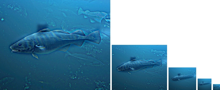
| Submarine + Fish | 4 | |||||
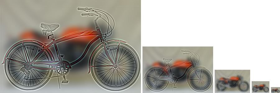
| Motorcycle + Bicycle | 6 | |||||
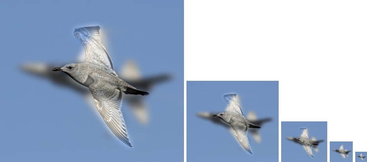
| Plane + Bird | 6.50 | |||||
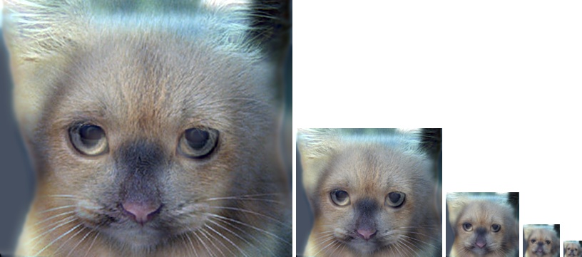
| Dog + Cat | 7 | |||||
| Marilyn + Einstein | 3 | |||||
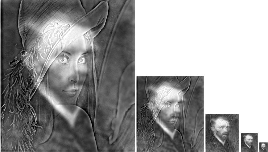
| Van Gogh + Lena | 4.50 |
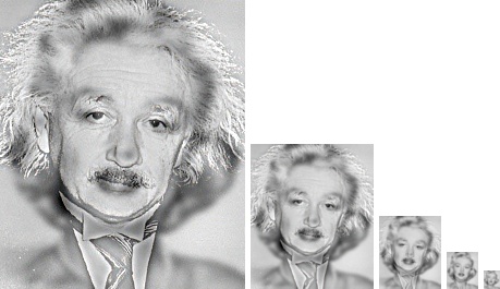
Below are the scale representations of the above pairs of hybrid images.
Extra: Slider Demo with Non-identical Cutoff Frequencies for G1 and G2
| Cutoff Frequency (G1) | Hybrid Image by Scale | Cutoff Frequency (G2) |
|---|---|---|
|
|
|
|
This demo allows the user to tune the cutoff frequencies for both the low-pass filtered image (Albert Einstein) and the high-pass filtered image (Marilyn Monroe). A higher cutoff frequency for the low-pass image increases the blurring effect, whereas doing so for the high-pass one serves to sharpen the image.
Try and see if you can produce a hybrid image that looks like Marilyn Monroe up close and Albert Einstein from a distance!