CS 6476 Project 1: Image Filtering and Hybrid Images
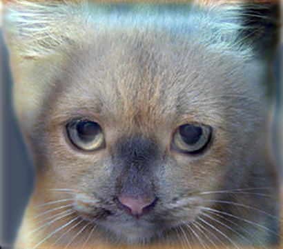
Figure 1: Hybrid image of a cat and a dog.
Part 1: Image Filtering [analogous to imfilter in Matlab]
Image filtering can be performed using two matrices. One matrix represents the image while the other represents the filter.
- Identify the dimensions of the image and the filter. The filter size is always represented by odd numbers.
- Pad the image with zeros in order to handle the edge pixels. The number of rows and columns to be added depends on the filter size.
- For each pixel in the image perform convolution by performing an element-wise multiplication with the filter.
- Add the values of the resultant matrix to obtain the value for the corresponding pixel in the output image.
- Repeat steps 3 and 4 for the entirety of the image
There are different ways to handle the edges in an image. One can either pad the image with zeros or mirror the values at the boundary of the image. I have padded the image with zeros.
Image Filtering Implementation
As we are supposed to be working with either gray scale or color images I have handled these cases seperately. The image with 1 channel is the gray scale image and the one having 3 channels (R,G,B) is the color image.
Part 1: Code
function output = my_imfilter(image, filter)
if(size(image,3) == 1)
    image_gray = zeros(size(image,1)+(size(filter,1)-1),size(image,2)+(size(filter,2)-1));
    image_gray(1 + ((size(filter,1)-1)/2): size(image,1)+((size(filter,1)-1)/2) ,
 1 + ((size(filter,2)-1)/2): size(image,2)+((size(filter,2)-1)/2) ) = image;
%padding for multiple channels - RGB
elseif (size(image,3) > 1)
    image_color = zeros(size(image,1)+(size(filter,1)-1),size(image,2)+(size(filter,2)-1),size(image,3));
    image_color(1 + ((size(filter,1)-1)/2): size(image,1) +((size(filter,1)-1)/2),
 1 + ((size(filter,2)-1)/2): size(image,2)+((size(filter,2)-1)/2),1:size(image,3)) = image;
%the output matrix
output = zeros(size(image));
%handling the case of a single channel in the image - grayscale image
if(size(image,3) == 1)
    %looping over the height of the image
    for i = 1 : size(image,1)
        %looping over the length of the image
        for j = 1 : size(image,2)
             %the output image to be displayed
             output_row = sum(image_gray(i:i+size(filter,1)-1, j:j+size(filter,2)-1).*filter);
             output(i,j) = sum(output_row);
        end
    end
%handling the case of multiple channels in the image (i.e. 3) - RGB image
elseif(size(image,3) > 1)
    %looping over the different channels
    for x = 1:size(image,3)
        %looping over the height of the image
        for i = 1 : size(image,1)
            %looping over the width of the image
            for j = 1 : size(image,2)
                %storing the output of the image in a single pixel by
                %summing over the columns and rows
                output_row = sum(image_color(i:i+size(filter,1)-1, j:j+size(filter,2)-1,x).*filter);
                output(i,j,x) = sum(output_row);
            end
        end
    end
end
end
Part 1: Results in a table
The following results represent the images on applying the different filter to the image - cat.bmp. On blurring the edges appear darkened and this occurs due to the padding with zeros.
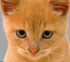
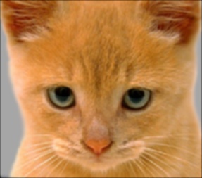
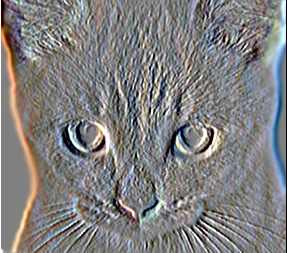
Figure 1: Identify Filter Figure 2: Small blur - Box filter Figure 3: Large blur - Gaussian filter Figure 4: Sobel filter 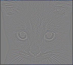
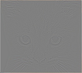
Figure 5: Discrete-Laplacian filter Figure 6: High Pass filter |
Part 2: Hybrid Images
To create an hybrid image, we require two images - image1 and image2
To remove the high frequencies from image 1 we blur it using a filter. Similarly, we remove the low frequencies to get the high frequencies from image2. We do this by first applying the filter to the image and then subtracting these low frequencies from the original image.
The hybrid image is obtained by summing image1 and image2
Part 2: Code
%removing high frequencies from image1
low_frequencies = my_imfilter(image1,filter);
%removing low frequencies from image2
high_frequencies = image2 - my_imfilter(image2,filter);
%combining the high and low frequencies
hybrid_image = low_frequencies + high_frequencies;
The standard deviation of the gaussian blur filter is given by the cut-off frequency. By varying this value we get the appropriate hybrid image for the given pair of images.
The cat-dog image pair - Image 1 is that of the dog and Image 2 that of the cat.
Cut-off frequency used is 7
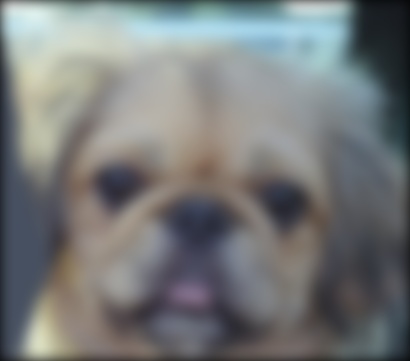
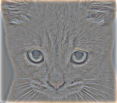
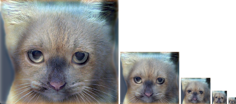
Image1 - Low Frequencies Image2 - High Frequencies Hybrid Image Scales of the Hybrid Image |
The marilyn-einstein image pair - Image 1 is that of the marilyn and Image 2 that of the einstein.
Cut-off frequency used is 2
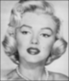
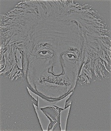
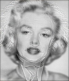
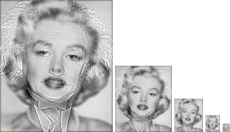
Image1 - Low Frequencies Image2 - High Frequencies Hybrid Image Scales of the Hybrid Image |
The bicycle-motorcycle image pair - Image 1 is that of the bicycle and Image 2 that of the motorcycle. Since these are contrasting images and the hybrid image was not ideal on using a single cut-off freqency, I used two different frequencies
%low frequency cut-off freqency
low_freq_cutoff_frequency = 9;
low_frequency_filter = fspecial('Gaussian',low_freq_cutoff_frequency*4+1,low_freq_cutoff_frequency )
%high freqency cut-off freqency
high_freq_cutoff_frequency = 5;
high_frequency_filter = fspecial('Gaussian',high_freq_cutoff_frequency*4+1,high_freq_cutoff_frequency )
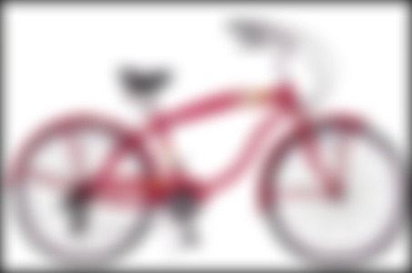
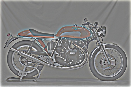
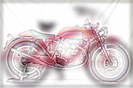
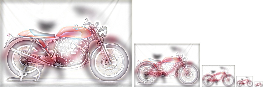
Image1 - Low Frequencies Image2 - High Frequencies Hybrid Image Scales of the Hybrid Image |
The bird-plane image pair - Image 1 is that of the bird and Image 2 that of the plane.
Cut-off frequency used is 4
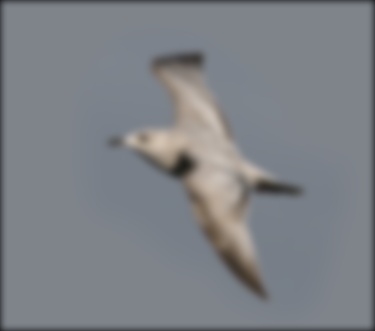
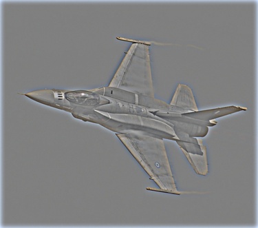
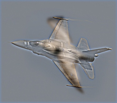
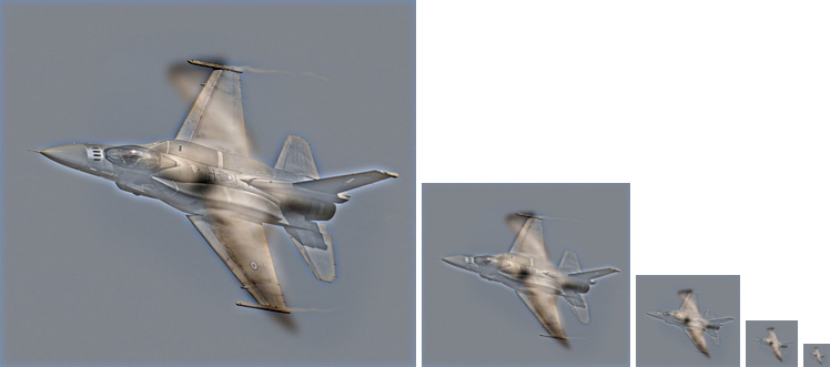
Image1 - Low Frequencies Image2 - High Frequencies Hybrid Image Scales of the Hybrid Image |
For the next set of images, I tried combinations of the images to obtain the final hybrid image. Clearly, as seen in the images below, one set of combination works better than the other.
First Combination: The fish - submarine image pair - Image 1 is that of the fish and Image 2 that of the submarine.
Cut-off frequency used is 7
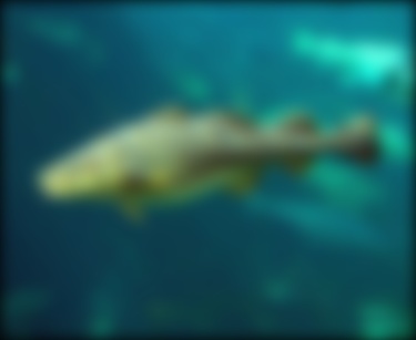
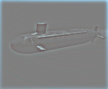
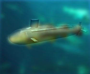
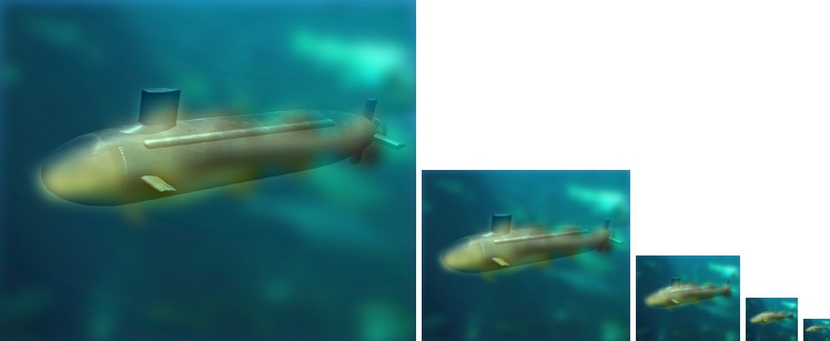
Image1 - Low Frequencies Image2 - High Frequencies Hybrid Image Scales of the Hybrid Image |
For the next set of images, I tried combinations of the images to obtain the final hybrid image. Clearly, as seen in the images below, one set of combination works better than the other.
Second Combination: The fish - submarine image pair - Image 1 is that of the submarine and Image 2 that of the fish.
Cut-off frequency used is 7
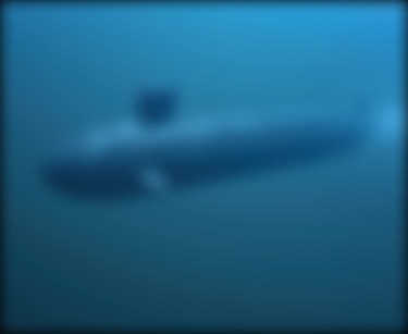
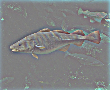
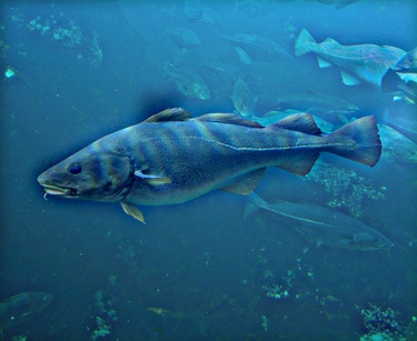
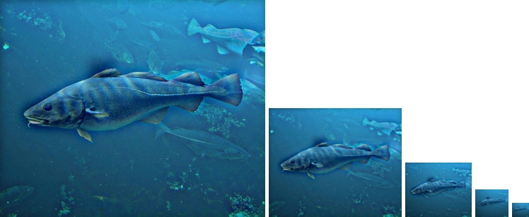
Image1 - Low Frequencies Image2 - High Frequencies Hybrid Image Scales of the Hybrid Image |
Through this experiment I observed that right image for the high frequency makes a lot of difference. Since this contains a lot of details, hence such images will be clearly visible when observed from nearby, but the details begin the fade as we move further from the image and hence the previously blurred out low frequency image becomes more evident. So the combination 1 clearly works out better than the combination 2 as the submarine has finer details than the fish and thus must be considered for the high frequency image. Hence the second combination is a failure.
Part 3: Interesting Results
An interesting hybrid image is that obtained from Barack Obama and John McCain.
Cut-off frequency used is 5.
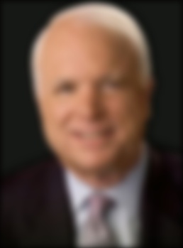
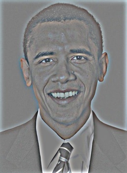

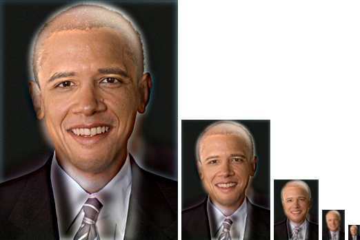
Image1 - Low Frequencies Image2 - High Frequencies Hybrid Image Scales of the Hybrid Image |
Another interesting hybrid image is that obtained from a cat and a mouse.
Cut-off frequency used is 3.
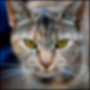
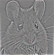
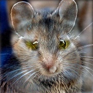
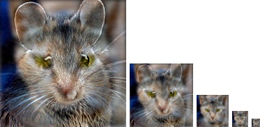
Image1 - Low Frequencies Image2 - High Frequencies Hybrid Image Scales of the Hybrid Image |
This hybrid depicts the images obtained of an Afghan girl when she was young and then years later. When looked at closely the image depicts the older person showing lines on the face,
but from a distance these details blur out and the image of the younger girl is more smoother.
Cut-off frequency used is 5.
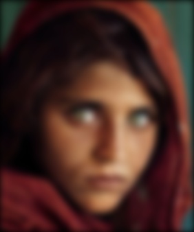
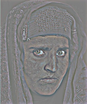
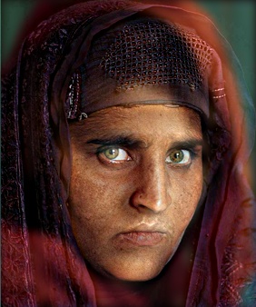
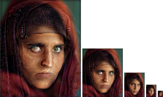
Image1 - Low Frequencies Image2 - High Frequencies Hybrid Image Scales of the Hybrid Image |
This hybrid depicts the images obtained of the same land during summer and winter. This image was interesting because of the contrast in colors. As we move away from the image the land during winter becomes more evident.
Cut-off frequency used is 4.
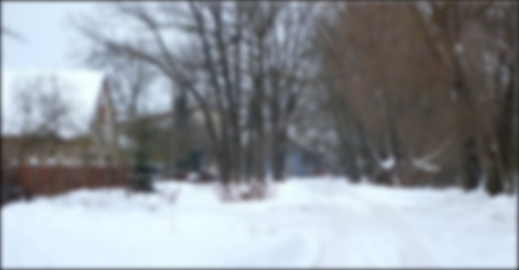
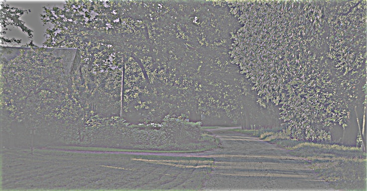
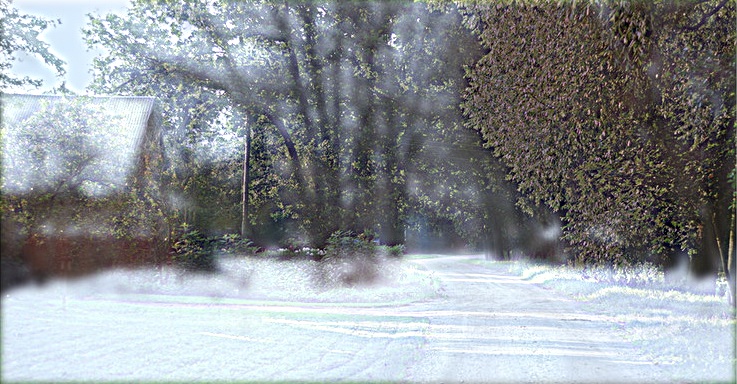
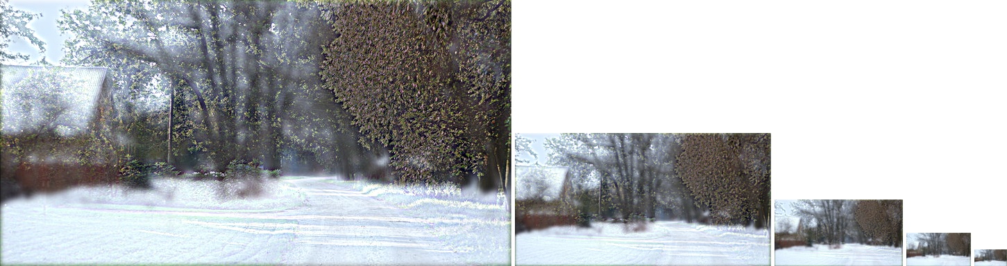
Image1 - Low Frequencies Image2 - High Frequencies Hybrid Image Scales of the Hybrid Image |
The images above (in Part 3) have been taken from projects published online. Only the individual images have been taken from these projects. The filtering and hybrid image is generated using the my_imfilter.m and proj1.m respectively. The links from where these images were obtained are http://students.cec.wustl.edu/~jwaldron/559/Project1/ and http://students.cec.wustl.edu/~billchang/cse559/project1/
Conclusion
The project deals with studying the effects of different filters on the image and formation of hybrid images. By setting an appropriate cut-off frequency we can obtain a good hybrid image.