Shaswat Shah

Project 1: Image Filtering and Hybrid Images

The goal of this assignment is to write an image filtering function and use it to create hybrid images using a simplified version of the SIGGRAPH 2006 paper by Oliva, Torralba, and Schyns. Hybrid images are static images that change in interpretation as a function of the viewing distance.

Image Filtering

Image filtering (or convolution) is a fundamental image processing tool. Here, we implemented my_imfilter() in Matlab which replicates the functionality of built-in imfilter(). Specifically, it is designed to handle the following cases:

1. Both RGB and grayscale images of any resolution are valid inputs
2. Any rectangular filter with odd filter width and odd filter height is a valid filter
3. The output after filtering should be the same size as the input image. For this pad the image with zeros at the boundaries as default behavior
4. (Extra) my_imfilter() also works with circular, symmetric and replicate padding just like the built-in imfilter() with the corresponding parameters in the function call

The filtering algorithm can be summarized as follows:

1. Pad image input by (filter dimension - 1) / 2 along x and y axes. Alternative padding methods can also be used here
2. For each output pixel per channel, compute the correlation as described below
3. To get output value for that pixel and channel, take the element-wise product of the filter and the subarray of the image obtained by superimposing the filter with its center as the output pixel in the given channel and compute the sum of all entries of the matrix
4. Return the output image

The following code snippet demonstrates the core functionality of my_imfilter():

function output = my_imfilter(image, filter, padval)
% Modified from
% function output = my_imfilter(image, filter)

[m, n] = size(filter);
[imy, imx, imz] = size(image);

% Default zero padding, can pass 'symmetric', 'circular'
% and 'replicate' as padval for corresponding padding
if nargin < 3
    padval = 0; % Does zero padding
end

padded = padarray(image, [(m - 1) / 2, (n - 1) /2], padval);

output = zeros(size(image));

for z = 1:imz
    for x = 1:imx
        for y = 1:imy
            output(y, x, z) = sum(sum(padded(y : y + m - 1, x : x + n - 1, z) .* filter));
        end
    end
end

Image Filtering Results

The images from left to right, top to bottom are:

1. Original Image
2. Identity filter output
3. Simple blur filter output
4. Large Gaussian blur filter output
5. Sobel filter output
6. High pass filter output
7. High pass filter (alternative) output

Hybrid Images

Hybrid images are static images that change in interpretation as a function of the viewing distance. The basic idea is that high frequency tends to dominate perception when it is available, but, at a distance, only the low frequency (smooth) part of the signal can be seen. By blending the high frequency portion of one image with the low-frequency portion of another, you get a hybrid image that leads to different interpretations at different distances.

A hybrid image is the sum of a low-pass filtered version of the one image and a high-pass filtered version of a second image. There is a free parameter, which can be tuned for each image pair, which controls how much high frequency to remove from the first image and how much low frequency to leave in the second image. This is called the "cutoff-frequency". In the paper it is suggested to use two cutoff frequencies (one tuned for each image) and you are free to try that, as well. In the starter code, the cutoff frequency is controlled by changing the standard deviation of the Gausian filter used in constructing the hybrid images.

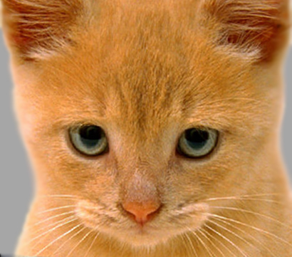
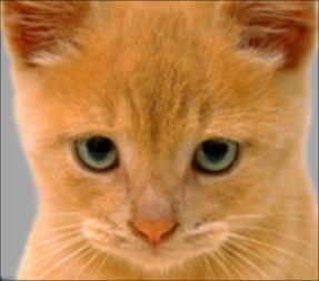
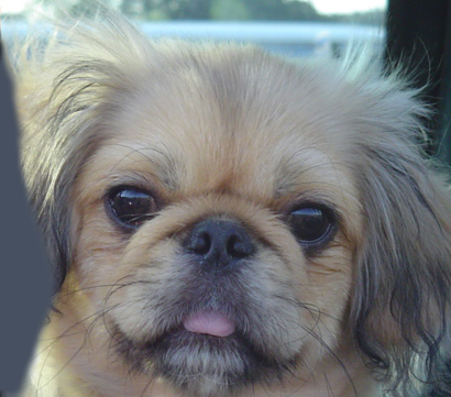
For the example shown at the top of the page, the two original images look like this:

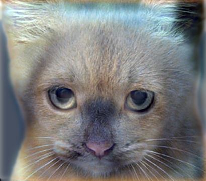
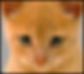
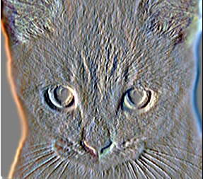
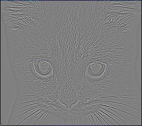
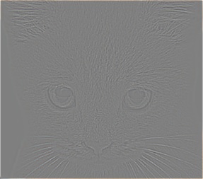
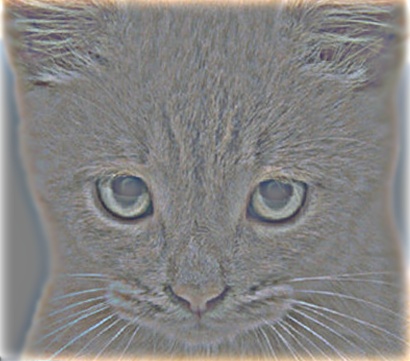
The low-pass (blurred) and high-pass versions of these images look like this:

The high frequency image is actually zero-mean with negative values so it is visualized by adding 0.5. In the resulting visualization, bright values are positive and dark values are negative.

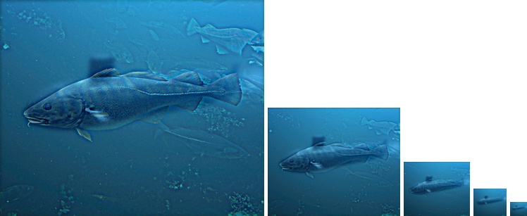
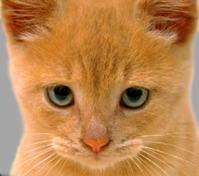
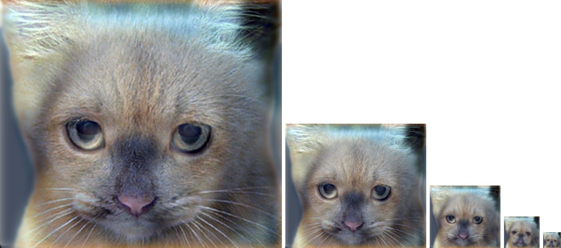
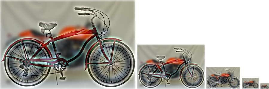
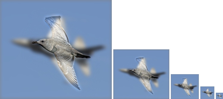
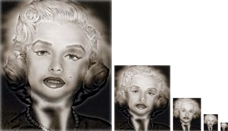
Adding the high and low frequencies together gives you the image at the top of this page. If you're having trouble seeing the multiple interpretations of the image, a useful way to visualize the effect is by progressively downsampling the hybrid image as is done below:

The following code snippet demonstrates how we create hybrid images:

image1 = im2single(imread('../data/cat.bmp'));
image2 = im2single(imread('../data/dog.bmp'));

cutoff_frequency = 6;
filter = fspecial('Gaussian', cutoff_frequency*4+1, cutoff_frequency);

low_frequencies = my_imfilter(image1, filter);
high_frequencies = image2 - my_imfilter(image2, filter);
hybrid_image = low_frequencies + high_frequencies;

Hybrid Image Results

For the provided 5 pairs of aligned images, we varied the free parameter "cutoff-frequency" to obtain good hybrid images.

Cat and Dog (Cutoff frequency=6)

Bicycle and Motorcycle (Cutoff frequency=5)

Bird and Plane (Cutoff frequency=6.5)

Marilyn and Einstein (Cutoff frequency=3.5)

Fish and Submarine (Cutoff frequency=3)