Project 1: Image Filtering and Hybrid Images

Image Filtering
I used MATLAB to implement the image filtering (convolution) function. Given a filter (2D matrix) and a digital image (3D matrix), the function outputs the filtered image result. The input image can be grayscale or color (the filter is applied separately for each image channel), and the filter can be any size with height and width both odd (this ensures that the center of the filter is unambiguously defined).
Filtering is implemented like 2D convolution in the spatial domain. The output image h is formed by applying the filter f centered at each pixel of the input image I.
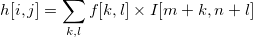
Formula used to compute each output pixel.
I implemented the filtering algorithm in the spatial domain for simplicity, however it is worth mentioning that it can alternatively be implemented in the frequency domain (Convolution Theorem) by doing: FFT inputs, multiply transforms, iFFT result. Although it was not implemented here, the frequency approach can reduce the number of computations for filtering.
Filtering on image edges is handled by first padding the image with pixels. There are several methods for padding images, however I used the reflection method (i.e. mirror image content over the boundaries as padding) because it introduces less noise into the output image. The images below show filter results for the reflection method and the clipping method (i.e. use zeros as padding).
Original image. |

Gaussian filter with reflection for padding. |
Gaussian filter with zeros for padding. |
Multiplying the filter with every image subwindow makes filtering computationally expensive. My implementation applies the filter at each position sequentially, so the run time is noticeably slow (several seconds for a small image). Although it is beyond the scope of this project, the image pixels could be filtered in parallel (e.g. using MATLAB's parfor operator) to achieve a performance speedup.
Another performance consideration is the use of separable filters. Whenever possible, the filter matrix should be factored into a vector product, and each vector applied to the image separately. Filtering is associative, so the final result will be the same. The table below shows a separated Gaussian filter applied to the image and demonstrates the associativity of filtering.
Original image. |

Separated Gaussian filter (vertical). |

Separated Gaussian filter (horizontal). |

Full Gaussian filter. |
The separated filter only requires a linear number of multiplications per image subwindow, whereas the combined filter takes a quadratic number of multiplications. I measured the running time (wall clock) for a combined (2D) Gaussian filter and a separated (1D) Gaussian filter, and got the following results.
| Gaussian Filter (25 x 25) | 11.345 seconds |
| Separated Gaussian Filter (25 x 1, 1 x 25) | 6.672 seconds |
For testing, I exported the output of my image filter and the output of MATLAB's built-in image filter ("imfilter"), and used numpy's allclose() operator to ensure that my image filtering function is working as expected for all of the provided input images.
Hybrid Images
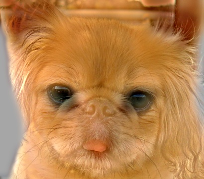
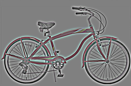
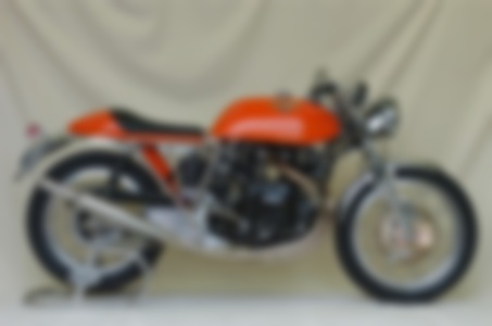
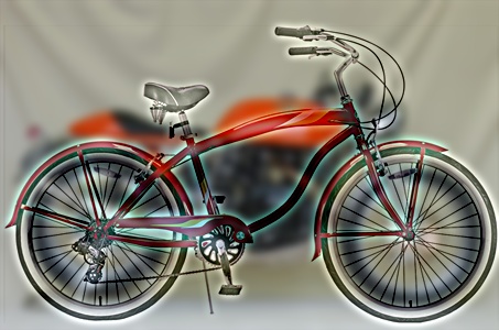
Given two input images, the low frequencies from the first image and high frequencies from the second image can be combined to form a single "hybrid image" that can be interpreted as either image at different viewing distances (especially if the objects in the input images are aligned). The high and low frequencies can be extracted using the image filtering algorithm from the previous section.

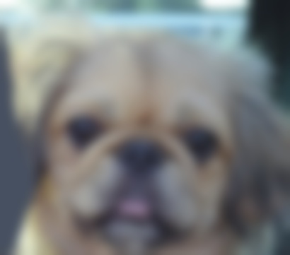
Input images. |
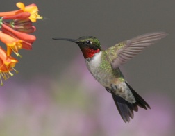
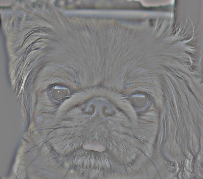
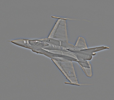
High frequencies. |
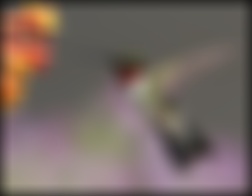
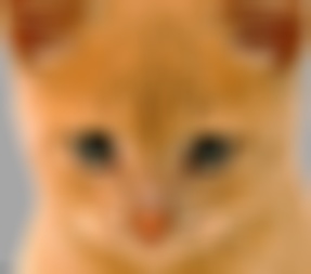
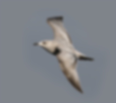
Low frequencies. |

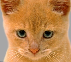
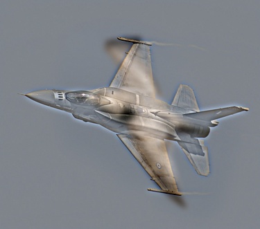
Hybrid image. |
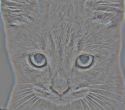
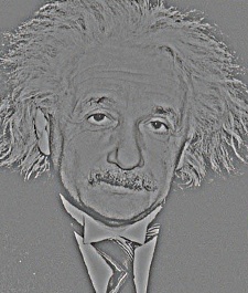
In the example above, high frequencies were removed from the dog image by applying a low pass (Gaussian blur) filter, and low frequencies were removed from the cat image by subtracting from it a low pass (Gaussian blur) filter applied to the same cat image. The standard deviation parameter for the Gaussian blur is 7 (found by trial and error of tuning and observing the hybrid image output). Note that the removal of the dog's high frequencies gives a blurring effect, and the colors are preserved. On the other hand, the removal of the cat's low frequencies leaves only fine lines, and most of the color is removed. Therefore adding the images together results in a hybrid image with colors dominant from the dog image.
In the next example, the same input images ("cat" and "dog") are used, but the order of the image pair is switched so that the dog's high frequencies and the cat's low frequencies are used to form the hybrid image. The same Gaussian filter with standard deviation 7 was used to filter the images. In this case, the colors in the cat image become dominant in the hybrid image.
High frequencies. |
Low frequencies. |
Hybrid image. |
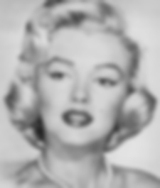
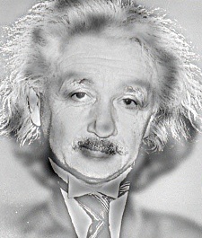
Several examples of hybrid images along with parameters used for each image pair:
Gaussian with standard deviation 7. |
Gaussian with standard deviation 4. |
Gaussian with standard deviation 3. |

Gaussian with standard deviation 7. |
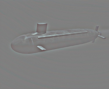
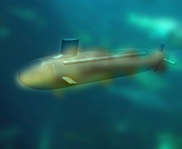
In the last hybrid image example, I noticed that the fish is almost too blurry to see from a distance. To fix this, I could decrease the Gaussian filter's standard deviation to make the fish less blurry, however with only one parameter this would have the double effect of removing more high frequencies from the submarine. Instead, I tried using two "cutoff frequency" parameters (one for each image) as suggested in the paper by Olivia et al. I made the fish image sharper by using a lower standard deviation of 4, and I kept the desired high frequencies in the submarine image by using a higher standard deviation of 9. The resulting image is shown below.
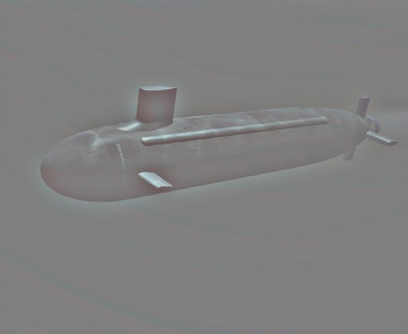

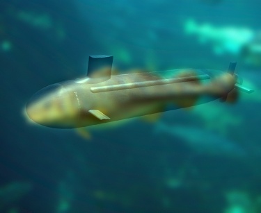
|