Project 1: Image Filtering and Hybrid Images
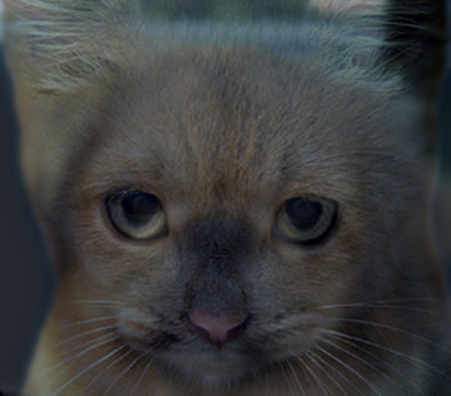
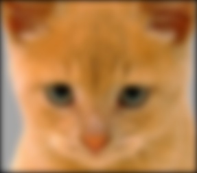
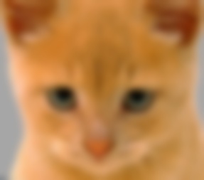
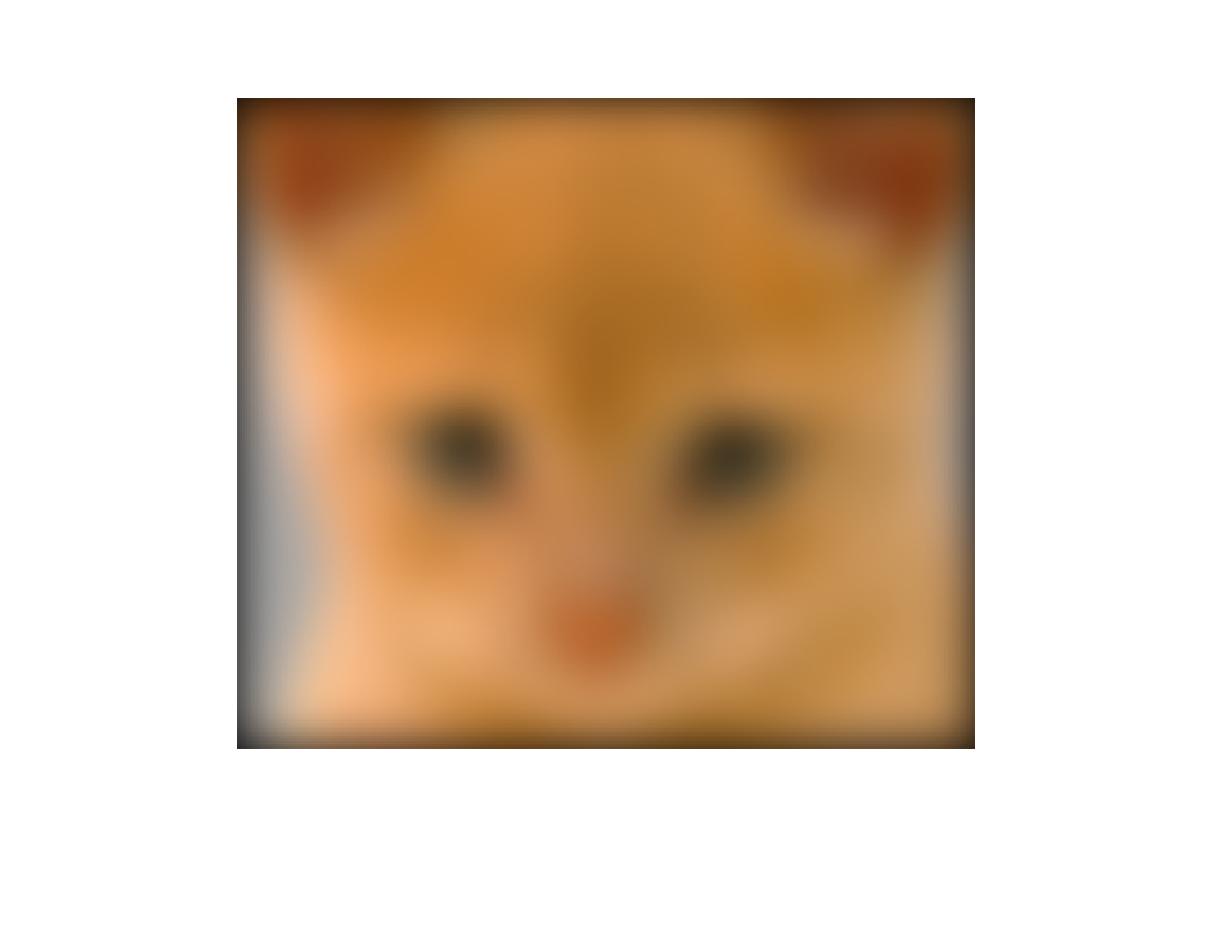
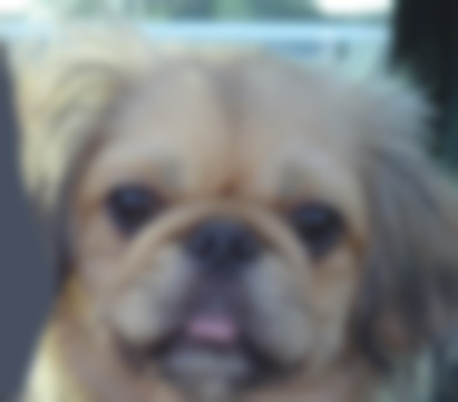
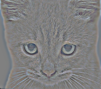
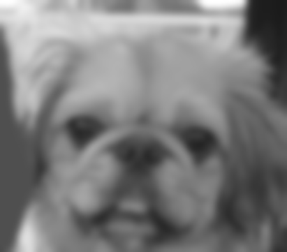
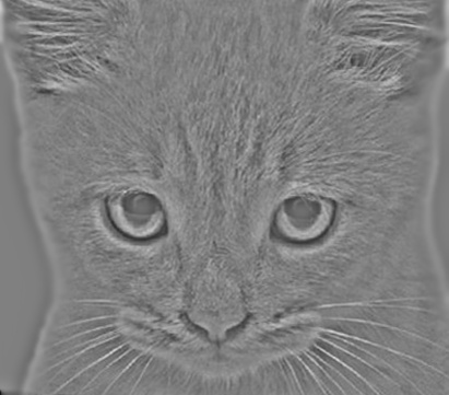
A blended image of a high-pass-filtered cat and a low-pass-filtered dog.
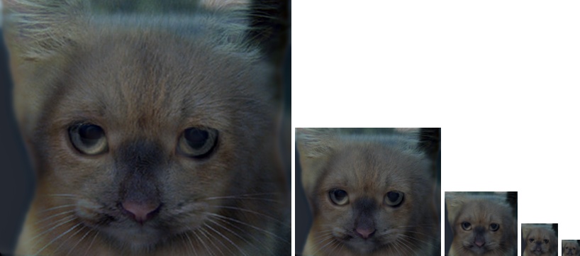
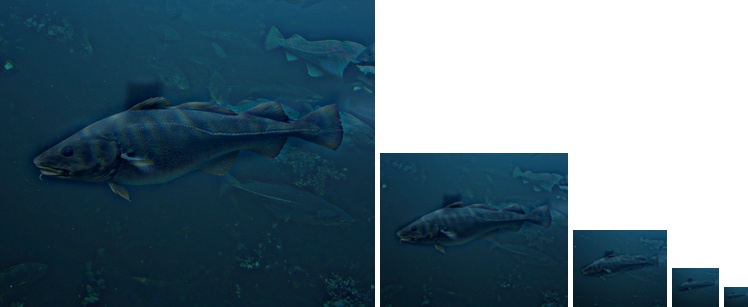
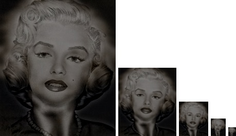
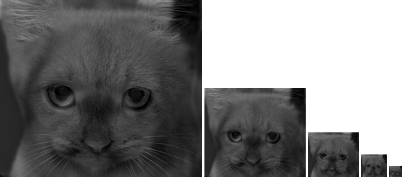
The goal of this assignment is to write an image filtering function and use it to create hybrid images using a simplified version of the SIGGRAPH 2006 paper by Oliva, Torralba, and Schyns. Hybrid images are static images that change in interpretation as a function of the viewing distance. The basic idea is that high frequency tends to dominate perception when it is available, but, at a distance, only the low frequency (smooth) part of the signal can be seen. By blending the high frequency portion of one image with the low-frequency portion of another, you get a hybrid image that leads to different interpretations at different distances. This document mainly discusses three key factors in the following order:
- Boundary conditions
- Spatial domain vs. Frequency domain
- Results
All the codes used for this assignment are included in the submitted folder, and some of the minor details regarding the implementation are omitted in this document.
Boundary issues
The author implemented two functions to take care of the boundary issues, which means the filter window falling off the original image when computing an element of the filtered image near the edge. First method is a clip filter, which adds extra zeros (black) to wrap around the original image. The second method is a mirroring method, which adds the pixels of the original image reflected across edges. Although there is no single best way to deal with this kind of a boundary issue, the mirroring method works best in most of the cases among the simple filtering techniques. The below shows the pseudo codes of the two implementations:
%clip filter
for channel = 1:nchannel
    tmp = [zeros(size(image, 1), add_size(2)) image(:, :, channel) zeros(size(image, 1), add_size(2))];
    f(:, :, channel) = [zeros(add_size(1), size(tmp, 2));
                  	tmp(:, :);
                  	zeros(add_size(1), size(tmp, 2))];
end
%mirror filter
for channel = 1:nchannel
    col_left = fliplr(image(:, 1:add_size(2), channel));
    col_right = fliplr(image(:, end - add_size(2) + 1:end, channel));
    f_col = [col_left image(:, :, channel) col_right];
    row_top = flipud(f_col(1:add_size(1), :));
    row_bottom = flipud(f_col(end-add_size(1) + 1:end, :));
    f(:, :, channel) = [row_top; f_col; row_bottom];
end
The figure below shows the results of the clip method (left) and the mirroring method (right) with the Gaussian blurring. As shown in the figure, the clip method has the black rim around the image the original image does not have. This is because we add zeros to compute the elements near the edges of the image. On the other hand, the mirroring method does not show an apparent discrepancy from the original image. However, the mirroring method is a rule-of-thumb, and it does not always show the better result over the clip method.
|
|
Spatial domain vs frequency domain
When we filter an image using convolution, there are two ways to do the operation: using spatial domain and frequency domain. A filtered image (h) can be created from an original image (f) and a filter (g) as follows:
% filter using the spatial domain
h = zeros(size(image));
for channel = 1:nchannel
    for m = 1:size(image, 1)
        for n = 1:size(image, 2)
            h(m, n, channel) = my_2dconv(g, f, m + add_size(1), n + add_size(2), channel);
        end
    end
end

% my function to call an element using 2d convolution
function hmn = my_2dconv(g, f, m, n, channel)
    hmn = 0;
    krange = (size(g, 1) - 1) / 2;
    lrange = (size(g, 2) - 1) / 2;
    for k = -krange:krange
        for l = -lrange:lrange
            hmn = hmn + g(k + krange + 1, l + lrange + 1) * f(m + k, n + l, channel);
        end
    end
end
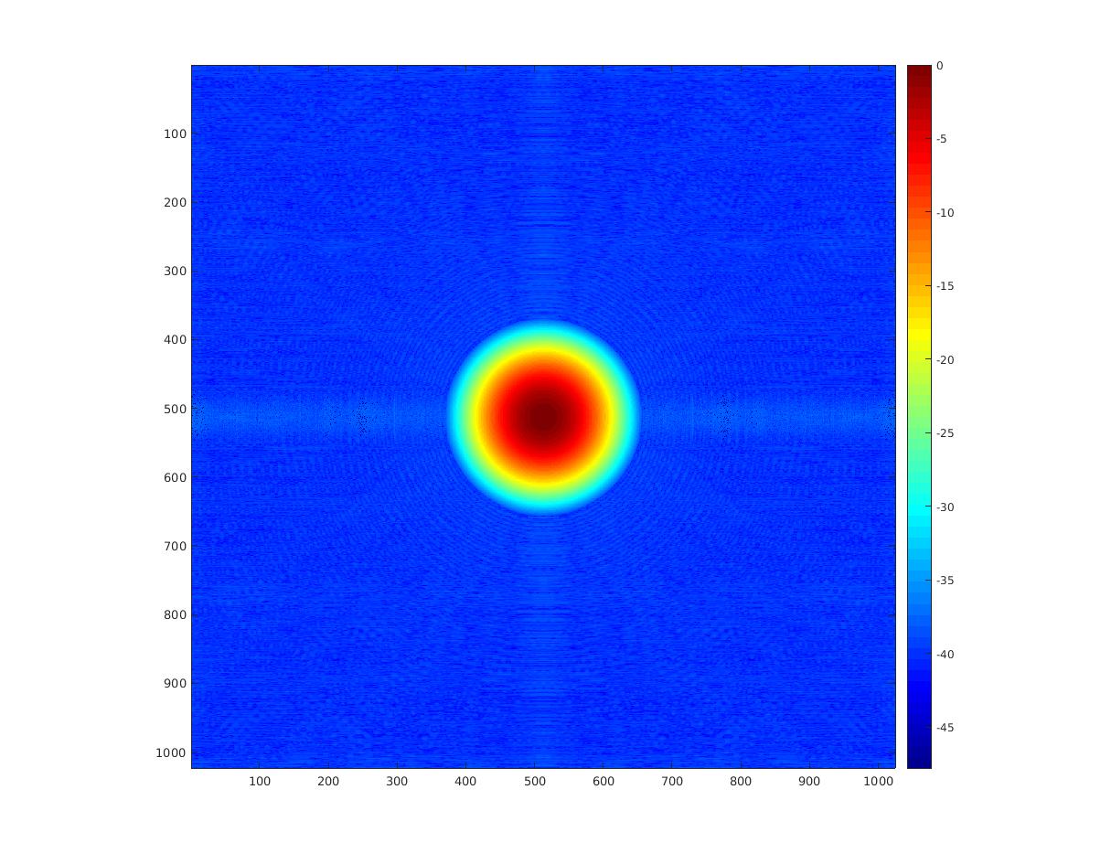
% create a low pass filter in a frequency domain
hs_low = 128;
fil_low = fspecial('gaussian', hs_low * 2 + 1, 10);
fftsize_low = 1024;
fil_fft_low = fft2(fil_low, fftsize_low, fftsize_low);
figure(8)
imagesc(log(abs(fftshift(fil_fft_low)))), axis image, colormap jet, colorbar;
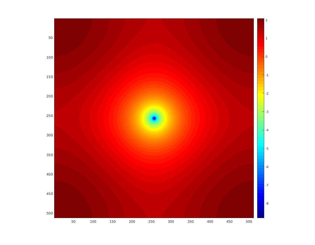
% create a high pass filter in a frequency domain
fftsize_high = 512;
laplacian_filter = [0 1 0; 1 -4 1; 0 1 0];
fil_fft_high = fft2(laplacian_filter, fftsize_high, fftsize_high);
figure(9)
imagesc(log(abs(fftshift(fil_fft_high)))), axis image, colormap jet, colorbar;
% create a low-pass-filtered image in a frequency domain
im_fft_low = zeros(fftsize_low, fftsize_low, size(test_image, 3));
im_fil_fft_low = zeros(fftsize_low, fftsize_low, size(test_image, 3));
im_fil_low = zeros(fftsize_low, fftsize_low, size(test_image, 3));
for i = 1:size(test_image, 3)
im_fft_low(:, :, i) = fft2(test_image(:, :, i), fftsize_low, fftsize_low);
im_fil_fft_low(:, :, i) = im_fft_low(:, :, i) .* fil_fft_low;
im_fil_low(:, :, i) = ifft2(im_fil_fft_low(:, :, i));
end
im_fil_low = im_fil_low(1 + hs_low:size(test_image, 1) + hs_low, 1 + hs_low:size(test_image, 2) + hs_low, :);
figure(10)
imshow(im_fil_low)
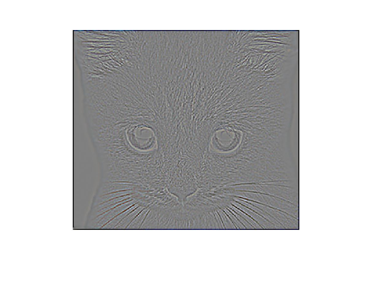
% creates a high-pass-filtered image in a frequency domain
hs_high = floor(size(laplacian_filter, 1) / 2);
im_fft_high = zeros(fftsize_high, fftsize_high, size(test_image, 3));
im_fil_fft_high = zeros(fftsize_high, fftsize_high, size(test_image, 3));
im_fil_high = zeros(fftsize_high, fftsize_high, size(test_image, 3));
for i = 1:size(test_image, 3)
im_fft_high(:, :, i) = fft2(test_image(:, :, i), fftsize_high, fftsize_high);
im_fil_fft_high(:, :, i) = im_fft_high(:, :, i) .* fil_fft_high;
im_fil_high(:, :, i) = ifft2(im_fil_fft_high(:, :, i));
end
im_fil_high = im_fil_high(1 + hs_high:size(test_image, 1) + hs_high, 1 + hs_high:size(test_image, 2) + hs_high, :);
figure(11)
imshow(im_fil_high + 0.5)
|
|
| Low-pass-filtered using a frequency domain, and reverted to a space domain | High-pass-filtered using a frequency domain, and reverted to a space domain |
|
|
| Gaussian low-pass-filter in a frequency domain | Laplacian high-pass-filter in a frequency domain |
Results
The my_imfilter implemented here
- supports grayscale and color images
- supports artitrary shaped filters as long as both dimensions are odd
- pads the input image with either zeros or to reflected image content, and
- returns a filtered image which is the same resolution as the input image.
The original data given for this assignment is a set of colored images, but you can test with grayscale images by commenting out these lines below in proj.m. The my_imfilter always checks the number of channels and returns an image that has the same number of channels.
% test grayscale
image1 = rgb2gray(double(image1));
image2 = rgb2gray(double(image2));
All the images are resized to the ones whose dimensions are odd in both directions.
% resize to odd resolutions if needed
if(mod(size(image1, 1), 2) == 0 || mod(size(image1, 2), 2) == 0)
    output_size(1) = size(image1, 1) - mod(size(image1, 1), 2) + 1;
    output_size(2) = size(image1, 2) - mod(size(image1, 2), 2) + 1;
    image1 = imresize(image1, output_size);
end
if(mod(size(image2, 1), 2) == 0 || mod(size(image2, 2), 2) == 0)
    output_size(1) = size(image2, 1) - mod(size(image2, 1), 2) + 1;
    output_size(2) = size(image2, 2) - mod(size(image2, 2), 2) + 1;
    image2 = imresize(image2, output_size);
end
You can choose how to pad the image using the switch below (which lives in my_imfilter.m)
boundary_mode = 1; % 0:zeros, 1:reflect
|
|
|
|


|
|
|
|
|
|

|
|
| High Pass | Low Pass | |
| CatDog | 8 | 5 |
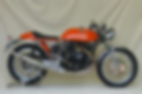
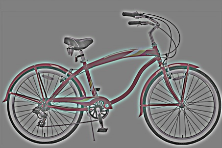
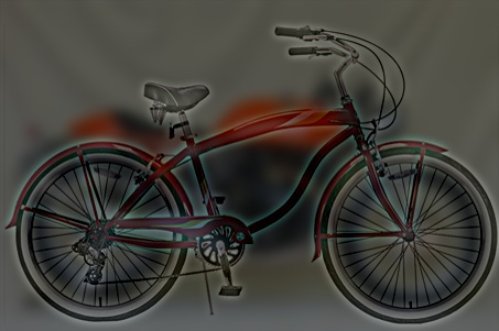
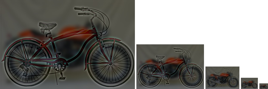
| Bi-MotorCycle | 4 | 6 |
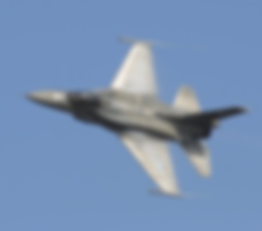
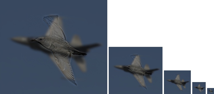
| BirdPlane | 4 | 4 |
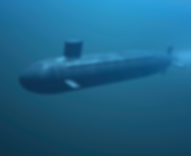
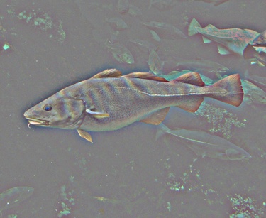
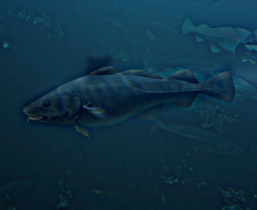
| FishSubmarine | 6 | 3 |
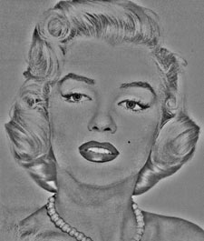
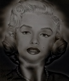
| MarilynEinstein | 6 | 4 |
function output = my_imfilter(image, filter)
    % This function is intended to behave like the built in function imfilter()
    % See 'help imfilter' or 'help conv2'. While terms like "filtering" and
    % "convolution" might be used interchangeably, and they are indeed nearly
    % the same thing, there is a difference:
    % from 'help filter2'
    %    2-D correlation is related to 2-D convolution by a 180 degree rotation
    %    of the filter matrix.

    % Your function should work for color images. Simply filter each color
    % channel independently.

    % Your function should work for filters of any width and height
    % combination, as long as the width and height are odd (e.g. 1, 7, 9). This
    % restriction makes it unambigious which pixel in the filter is the center
    % pixel.

    % Boundary handling can be tricky. The filter can't be centered on pixels
    % at the image boundary without parts of the filter being out of bounds. If
    % you look at 'help conv2' and 'help imfilter' you see that they have
    % several options to deal with boundaries. You should simply recreate the
    % default behavior of imfilter -- pad the input image with zeros, and
    % return a filtered image which matches the input resolution. A better
    % approach is to mirror the image content over the boundaries for padding.

    % % Uncomment if you want to simply call imfilter so you can see the desired
    % % behavior. When you write your actual solution, you can't use imfilter,
    % % filter2, conv2, etc. Simply loop over all the pixels and do the actual
    % % computation. It might be slow.
    %output = imfilter(image, filter);

    %%%%%%%%%%%%%%%%
    % Your code here
    %%%%%%%%%%%%%%%%
    if(mod(size(image, 1), 2) == 0 || mod(size(image, 2), 2) == 0)
        disp('Invalid Image Size');
    else
        fprintf('Image size is [%d, %d]\n', size(image, 2), size(image, 1))
    end
    g = filter;
    nchannel = size(image, 3);
    if(nchannel == 1)
        disp('processing a grayscale image ...');
    elseif(nchannel == 3)
        disp('processing a color image ...');
    else
        disp('Invalid nchannel');
    end

    boundary_mode = 1; % 0:zeros, 1:reflect
    add_size = [(size(g, 1) - 1) / 2, (size(g, 2) - 1) / 2];
    f = zeros(size(image, 1) + 2*add_size(1), size(image, 2) + 2*add_size(2));
    if(boundary_mode == 0)
        for channel = 1:nchannel
            tmp = [zeros(size(image, 1), add_size(2)) image(:, :, channel) zeros(size(image, 1), add_size(2))];
            %size_tmp = size(tmp)
            f(:, :, channel) = [zeros(add_size(1), size(tmp, 2));
                          tmp(:, :);
                          zeros(add_size(1), size(tmp, 2))];
        end
    elseif(boundary_mode == 1)
        for channel = 1:nchannel
            col_left = fliplr(image(:, 1:add_size(2), channel));
            col_right = fliplr(image(:, end - add_size(2) + 1:end, channel));
            %size_col_left = size(col_left)
            %size_col_right = size(col_right)
            %size_image = size(image)
            f_col = [col_left image(:, :, channel) col_right];
            %size_f_col = size(f_col)
            row_top = flipud(f_col(1:add_size(1), :));
            row_bottom = flipud(f_col(end-add_size(1) + 1:end, :));
            %size_row_top = size(row_top)
            %size_row_bottom = size(row_bottom)
            f(:, :, channel) = [row_top; f_col; row_bottom];
        end
    else
        disp('Invalid boundary mode');
    end
    h = zeros(size(image));
    for channel = 1:nchannel
        for m = 1:size(image, 1)
            for n = 1:size(image, 2)
                h(m, n, channel) = my_2dconv(g, f, m + add_size(1), n + add_size(2), channel);
            end
        end
    end
    output = h;
end

function hmn = my_2dconv(g, f, m, n, channel)
    hmn = 0;
    krange = (size(g, 1) - 1) / 2;
    lrange = (size(g, 2) - 1) / 2;
    for k = -krange:krange
        for l = -lrange:lrange
            hmn = hmn + g(k + krange + 1, l + lrange + 1) * f(m + k, n + l, channel);
        end
    end
end
Biography
Takuma Nakamura is a Ph.D. student working with Dr. Eric N. Johnson at the Unmanned Aerial Vehicle Research Facility at Georgia Tech in Atlanta. He started his undergraduate study at Tohoku University, Sendai, Japan in 2009 and received a Bachelor of Engineering in Mechanical and Aerospace Engineering in March 2013. The following August, he joined the graduate study program in the School of Aerospace Engineering at Georgia Tech. He received a Master of Science in Aerospace Engineering from Georgia Tech in August 2015 and is continuing in the PhD program. His research interests include the computer vision systems, autonomous flight control for UAVs, six-degrees-of-freedom flight simulation and modeling. He is also a licensed private pilot, and hobby drone operator.