Xiaobin Xiong

Project 1: Image Filtering and Hybrid Images

Content

1. Image Filtering
2. Hybrid Images
3. Extra Credit: Using FFT

1. Image Filtering

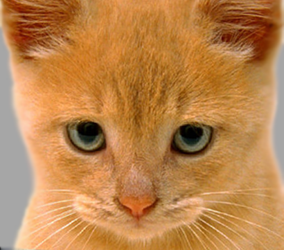
Image filtering is a fundamental image processing tool for various purposes, including smoothing, sharpening and edge detections. It always uses a collection of pixel values in the vicinity of each pixel to generate a new pixel value. Linear filter is one of the most commonly used filters. In the first part of this project, a linear filter function, called my_imfilter, is implemented to complete various filters. The cat image of Fig. 1 is the instance for testing. Both grayscale and color images can be used in this filter function. Arbitrary shaped filter matrices are supported as long as the dimensions of the matrices are odd, for which to eliminate ambiguity about the center of each filter matrix. For simplicity, the input image is padded with zeros and the filtered image will be of the same resolution as the input image.

The function takes an image matrix and a filter matrix as inputs. The image matrix is 3 dimensions of N_rows*N_columns*N_c which represents numbers of rows, columns and channels respectively. A grayscale image has only one channel of gray values. And a color image usually has three channels of Red, Green and Blue (RGB). While the filter matrix is only of two dimensions. To begin with, the function declaration is

function output = my_imfilter(image, filter)

And the dimensions of both matrices are measured.

[ N_rows, N_columns, N_c ] = size(image);
[ N_r_filter, N_c_filter] = size(filter);

To apply the filter on the image, a padded image, called Pad_image, is created first. The resolution of Pad_image should be bigger than the input image so that each pixel on the boundaries of the input image still has neighbors in its vicinity when applying filter matrix on this pixel. Pad_image should have at least half of the number of columns in filter matrix more than the number of columns of the input image in both left column and right column directions, and should have at least half of the number of rows in filter matrix more than the number of columns of the input images in both upper and lower row directions. For instance, the filter matrix is of 5 by 5, and the resolution of the input image is 1960*1080. Adding 2 rows of zeros above, 2 rows of zeros below, 2 columns of zeros to the left and 2 columns of zeros to the right of the input image will generate the Pad_image, the resolution of which would be 1964*1084. The following code is even easily to explain this.

boud_row = floor(N_r_filter/2);
boud_col = floor(N_c_filter/2);
Pad_image = zeros(N_rows + 2*boud_row, N_columns + 2*boud_col, N_c);
Pad_image(boud_row + 1:boud_row+N_rows,boud_col + 1:boud_col+N_columns,:) = image;

Then we can iterate the filtering process on each pixel of the image part in Pad_image, and save the pixel values into the output image called output. A temporary matrix called Temp_matrix to locate the vicinity of each pixel. The sum of all the values in the element-wise multiplication of Temp_matrix and the filter matrix will be the filtered value for this pixel. As the iteration should spread from each row, column and channel, three for loops are implemented.

output = zeros(N_rows,N_columns,N_c);
for i = boud_row+1: boud_row + N_rows
    for j = boud_col +1:boud_col + N_columns
        for k = 1:N_c
            Temp_matrix = Pad_image(i-boud_row:i+boud_row,j-boud_col:j+boud_col,k);
            output(i-boud_row,j-boud_col,k) = sum(sum(Temp_matrix.*filter));
        end
    end        
end

Having all the code in a single .m file, we have the my_imfilter function. To test this filter function, identity_file, blur_filter, large_blur_image, sobel_filter, laplacian_filter and high_pass_filter are taken as input filters respectively. The results are listed as follows.

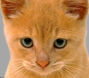
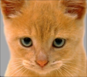
Fig. 2.1 Identity Filter.	Fig. 2.2 Blur Filter.	Fig. 2.3 Large Blur Filter.
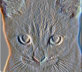
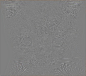
Fig. 2.4 Sobel Filter.	Fig. 2.5 Laplacian Filter.	Fig. 2.6 High Pass Filter.

2. Hybrid Images

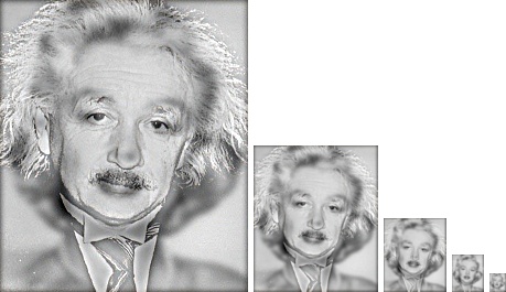
Given a cutoff-frequency, we can remove higher frequency in one image to generate a low-pass filtered image, or leave higher frequency in one image to generate a high-pass filtered image. Overlaying a low-pass filtered image on a high-pass filtered image will potentially generate a hybrid image. Human eyes capture the high-pass filter image at a close distance. While at a far distance, the low-pass filter image is easily captured from the hybrid image. Down-sampled hybrid images are used for visualization from different distances. In order to merge paired images reasonably together into a hybrid image, objects in the each pair should be aligned to similar positions in the image frame. In this project, five pairs of images are provided, including cat/dog, bicycle/motorcycle, bird/plane, fish/submarine and Einstein/Marilyn. Let's first use the images of Marilyn and Einstein to demonstrate how the hybrid image is generated, and then use the same method to generate hybrid images for the other pairs.

The original images of Marilyn and Einstein look like in Fig. 3.1 and 3.2.

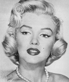
Fig. 3.1 Image of Marilyn.

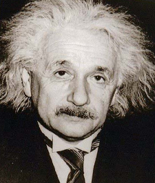
Fig. 3.2 Image of Einstein.

We will first blur Einstein and remove blured Marilyn (to generate a high pass filtered Marilyn) to generate a hybrid image of Marilyn/Einstein, which would look like Marilyn at close distance and like Einstein at a larger distance. A gaussian filter is used to generate low-pass and high-pass filtered images. Using the cutoff-frequency as the standard diviation in pixels, the gaussian filter is generated as follows.

cutoff_frequency =4.5; 
filter = fspecial('Gaussian', cutoff_frequency*4+1, cutoff_frequency);

Assuming image1 is the image of Einstein and image2 is that of Marilyn, we can get a blurred Einstein called low_frequencies by applying the gaussian filter to image1. Cleverly, we can thus get a high-pass filtered Marilyn called high_frequencies by using the original Marilyn subtract a blurred Marilyn. Combining the blurred Einstein like Fig. 3.3 and the high-passed Marilyn like Fig. 3.4, we finally generate a hybrid image in Fig. 3.5.

low_frequencies = imfilter(image1,filter);
high_frequencies = image2 - imfilter(image2,filter);
hybrid_image = (low_frequencies + high_frequencies);

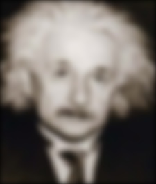
Fig. 3.3 Blurred Einstein.

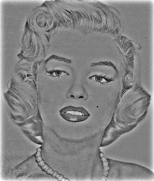
Fig. 3.4 High-passed Marilyn.

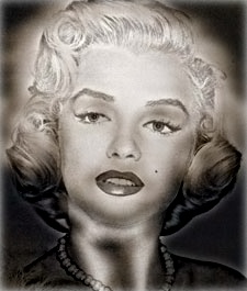
Fig. 3.5 Hybrid Marilyn/Einstein.

Using the down-sampled hybrid images in Fig. 3.6, we visualize the Marilyn/Einstein hybrid image as if we look at it at different distances. Just like that we mentioned before, the hybrid image looks like Marilyn at first and then looks like Einstein at farther distances.

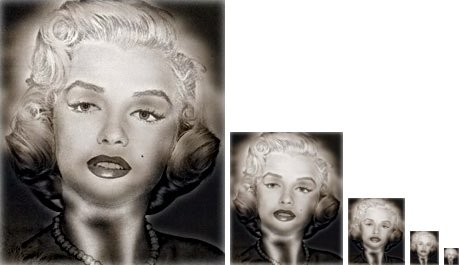
Similarly, hybrid images of Einstein/Marilyn (reversed), cat/dog, bicycle/motorcycle, bird/plane, and fish/submarine are also generated by the same procedure. Please enjoy the results in the following figures. The only parameter to change is the cutoff-frequency. Using binary search, optimum cutoff-frequencys are list in Table 1 at the bottom of this section.

Fig. 4.1 Blurred Marilyn.

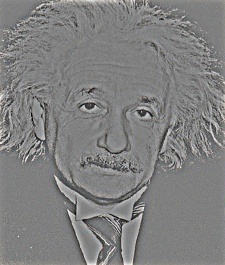
Fig. 4.2 High-passed Einstein.

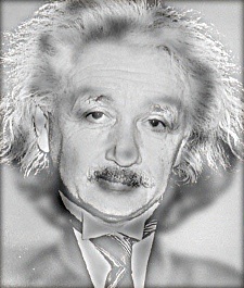
Fig. 4.3 Hybrid Einstein/Marilyn.

Fig. 5.1 Cat.

Fig. 5.2 Dog.

Fig. 5.3 Blurred Dog.

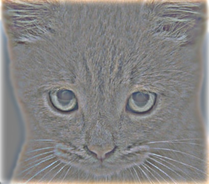
Fig. 5.4 High-passed Cat.

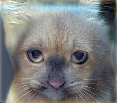
Fig. 5.5 Hybrid Cat/Dog.

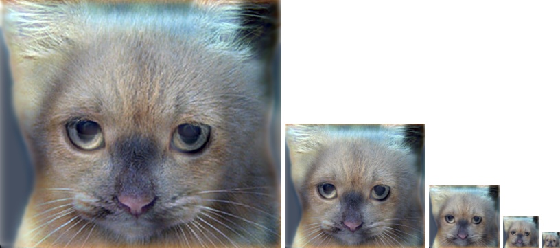
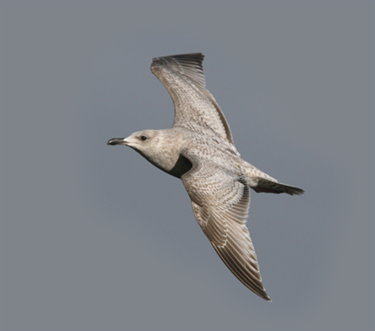
Fig. 6.1 Bird.

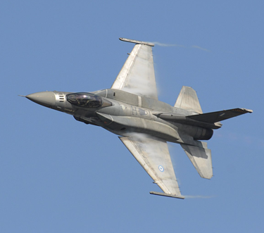
Fig. 6.2 Plane.

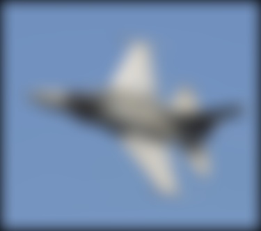
Fig. 6.3 Blurred Plane.

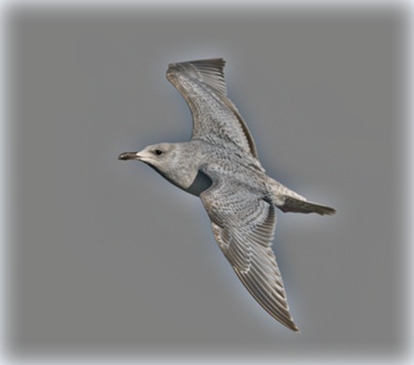
Fig. 6.4 High-passed Bird.

Fig. 6.5 Hybrid Bird/Plane.

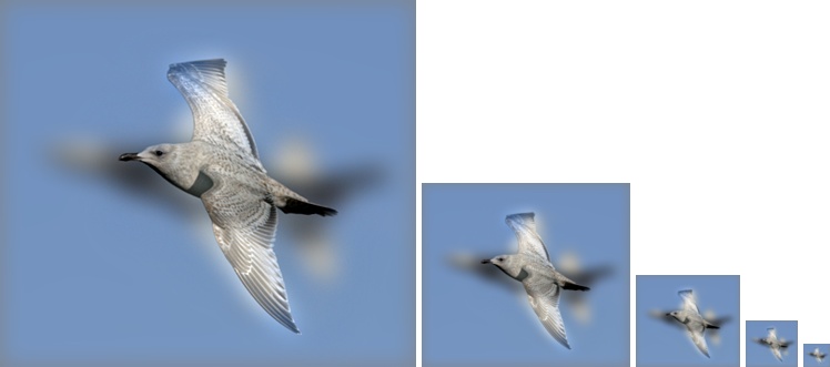
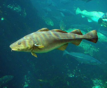
Fig. 7.1 Fish.

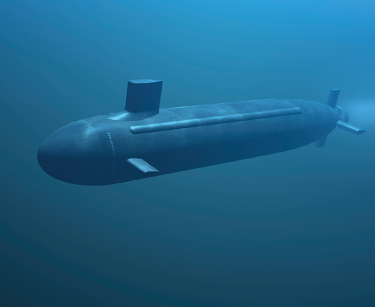
Fig. 7.2 Submarine.

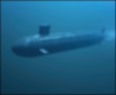
Fig. 7.3 Blurred Submarine.

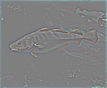
Fig. 7.4 High-passed Fish.

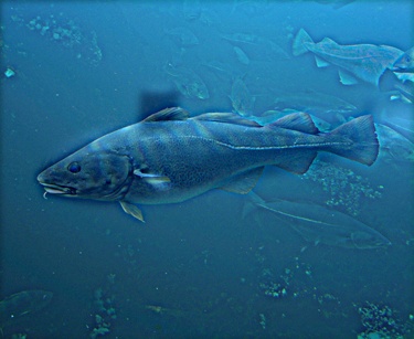
Fig. 7.5 Hybrid Fish/Submarine.

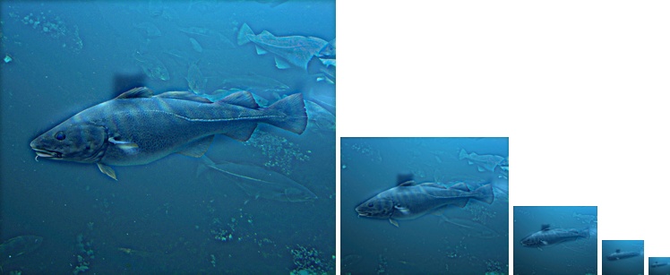
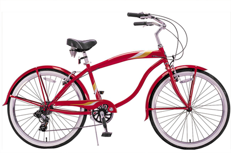
Fig. 8.1 Bicycle.

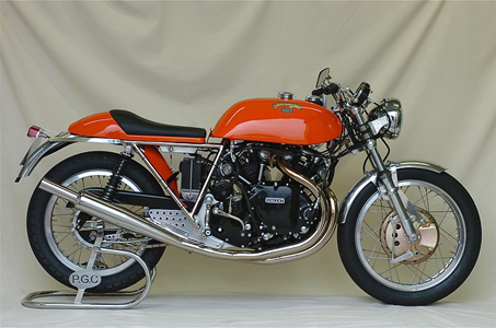
Fig. 8.2 Motorcycle.

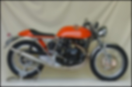
Fig. 8.3 Blurred Motorcycle.

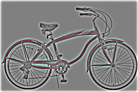
Fig. 8.4 High-passed Bicycle.

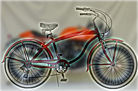
Fig. 8.5 Hybrid Bicycle/Motorcycle.

Table 1 Cut-off frequencies for each hybrid image pairs.

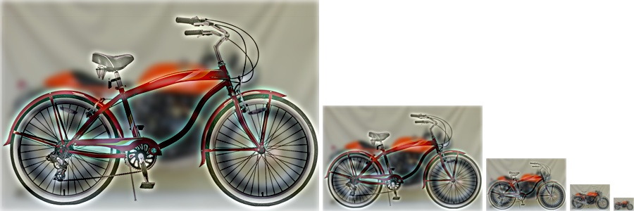
Marilyn/Einstein	Einstein/Marilyn	Cat/Dog	Bicycle/Motorcycle	Bird/Plane	Fish/Submarine
4.5	3	7	4.5	11	3.5

3. Extra Credit: Using FFT

In this last section, I will first use the convolution theorem to implement filtering in Fourier space. And then using the same method to create hybrid images without using filtering.

Fourier transformation is often used to interpret data in frequency domain. Maltab offers fft2 function to extract frequency information from images. To implement filtering in Fourier space, we will use the convolution theorem: Convolution in spatial domain is equivalent to multiplication in frequency domain. First, a image is read and normalized. FFT2 is applied to RGB three channels.

image1 = double(imread('../data/dog.bmp'))/255;
[rows,cols,cn] = size(image1);
fftsize = 1024;
fft1r =fft2(image1(:,:,1),fftsize,fftsize);
fft1g =fft2(image1(:,:,2),fftsize,fftsize);
fft1b =fft2(image1(:,:,3),fftsize,fftsize);

Then the filer is also interpreted in Fourier space. The half size of the filter size half_fs should be recorded to remove padding in the next steps.

filter_size = 25;
large_1d_blur_filter = fspecial('Gaussian', filter_size, 10);
half_fs = floor(filter_size/2);
filter_fft = fft2(large_1d_blur_filter,fftsize,fftsize);

Multiplication of each channel and the filter in the frequency domain will provide filtered in each channel. Inversing the FFT using ifft2 and combining the three channels, we should be able to generate a filtered image called im1.

im_fil_fft_r = fft1r.*filter_fft;
im_fil_fft_g = fft1g.*filter_fft;
im_fil_fft_b = fft1b.*filter_fft;
im1r = ifft2(im_fil_fft_r);
im1g = ifft2(im_fil_fft_g);
im1b = ifft2(im_fil_fft_b);
im1 = zeros(rows,cols,cn);
im1(:,:,1) = im1r(1+half_fs:rows+half_fs,1+half_fs:cols+half_fs);
im1(:,:,2) = im1g(1+half_fs:rows+half_fs,1+half_fs:cols+half_fs);
im1(:,:,3) = im1b(1+half_fs:rows+half_fs,1+half_fs:cols+half_fs);

Using the Dog image as an example, we can compare this method with my_imfilter function. Fig. 9.1 shows the filtered image using FFT, and Fig. 9.2 is the image using my_imfilter function. As the two filtered images are identical, the convolution theorem is verified.

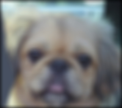
Fig. 9.1 Blur filtered dog using FFT.

Fig. 9.2 Blur filtered dog using my_imfilter.m.

Using the same method we can create hybrid images as well. Fig. 10 shows the hybrid image of Cat/Dog generated by using FFT. Code implementation can be found in folder code/FFT4HybridImage.m.