Project 2: Local Feature Matching
Feature detection and matching are an essential component of many computer vision applications. They are used in a variety of applications like image alignment, object recognition, 3D reconstruction, motion tracking, indexing and content-based retrieval, robot navigation etc. A good feature would lead to unambiguous matches in other images. Local features are useful because they are robust to occlusion and clutter, can differentiate a large database of objects, are large in number (for each image), efficient and can exploit different types of features in different situations.
The first kind of feature that you may notice are specific locations in the images, such as mountain peaks, building corners, doorways, or interestingly shaped patches of snow. These kinds of localized feature are often called keypoint features or interest points (or even corners) and are often described by the appearance of patches of pixels surrounding the point location. Algorithms that extract these features are Harris detector, Shi and Tomasi detector, Level curve curvature detector, Hessian feature strength measures detector, SUSAN and FAST. Another class of important features are edges, e.g., the profile of mountains against the sky. These kinds of features can be matched based on their orientation and local appearance (edge profiles) and can also be good indicators of object boundaries and occlusion events in image sequences. Edges can be grouped into longer curves and straight line segments, which can be directly matched or analyzed to find vanishing points and hence internal and external camera parameters. Algorithms to detect these features are Canny detector, Deriche detector, Differential filter, Sobel filter, Prewitt filter, Roberts cross detector. There are also blob detectors which can be detected by algorithms like Laplace of Gaussian, Difference of Gaussian, Determinant of Hessian, Maximally stable extremal regions (MSER) etc. There are other kinds of features like ridge features etc.
There are three main stages in the feature matching pipeline:
- Feature detection
- Feature description, and
- Feature matching
1. Feature detection
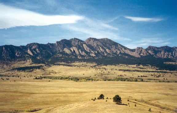
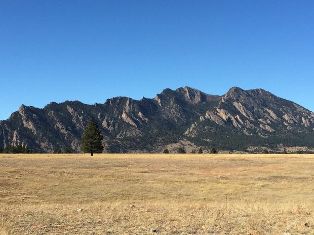
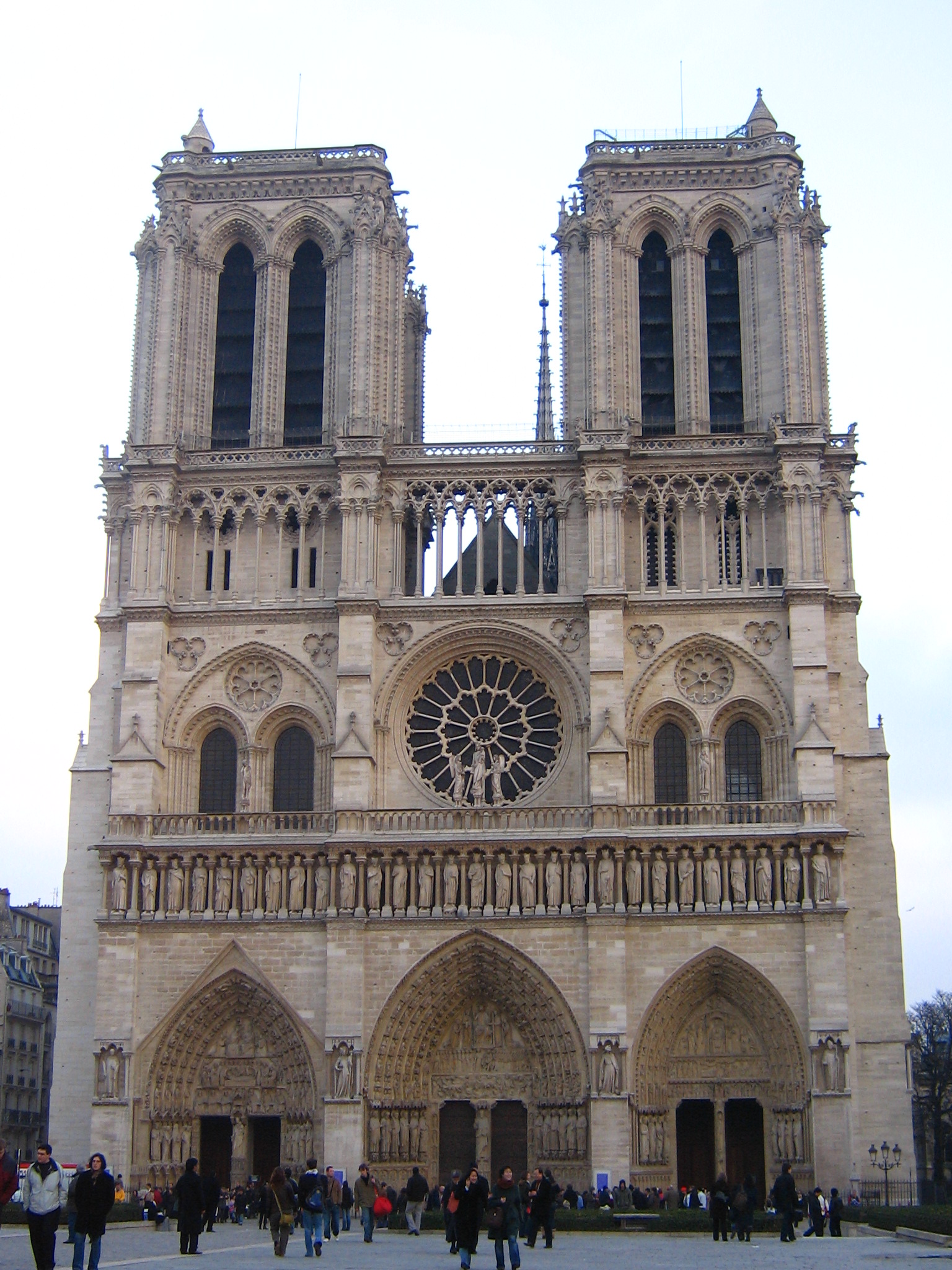
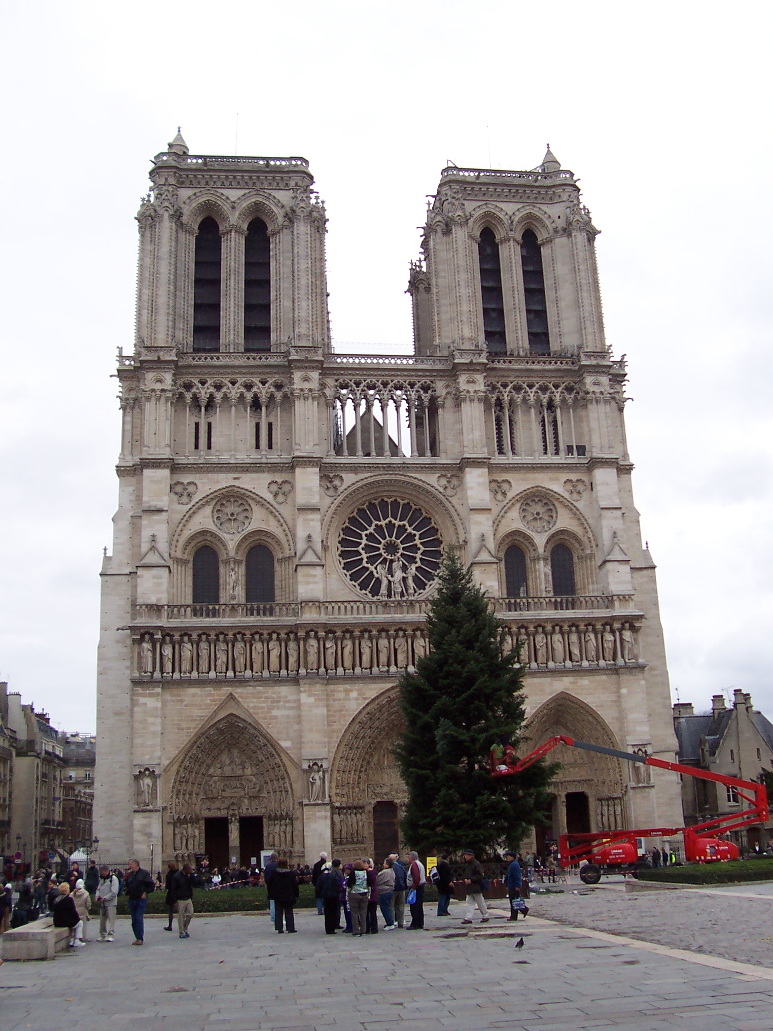
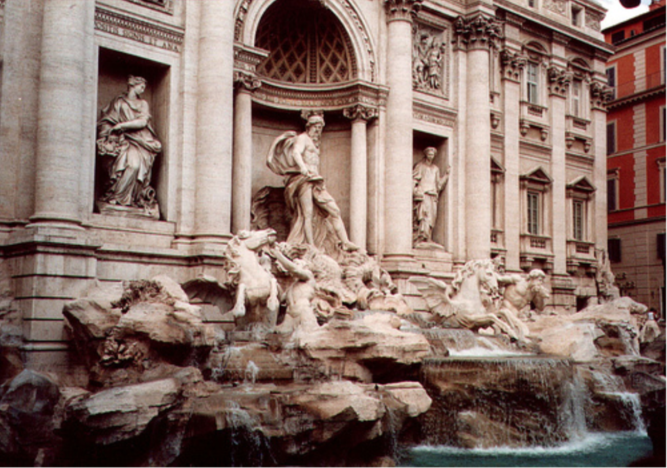
A good way to compare two pictures would be to compare every pixel or every small block of one picture to every small block of another picture and see if they match. But this method is very computationally expensive. And if you have images like the following:
|
we would mostly end up comparing a number of patches of sky and a number of patches of grass that look extremely similar. Images might undergo various transformations like scaling, translation, rotation or changing brightness and exposure etc. A naive way wouldn't be able to take these into consideration.
A better way to do this would be to extract features that have a greater chance of being unique, features that are invariant to these transformations. There are a number of ways to do this. In this project, I shall describe the Harris Corner detector, it's extension the Shi Tomasi detector and a few more extensions.
The Harris Corner detector is based on the understanding that corners are generally stable over variations of viewpoint. One can easily recognize a corner by looking at the intensity values in a small window. Shifting the window in any direction should yield a large change in appearance.
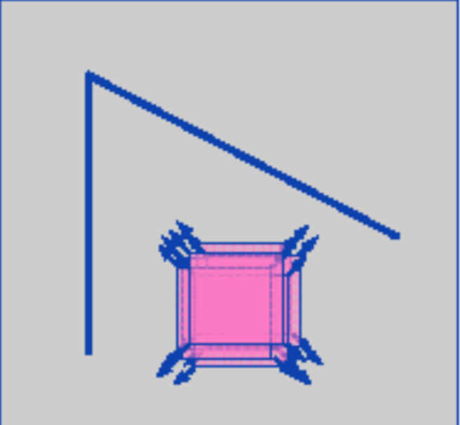
Flat region: no change in all directions |
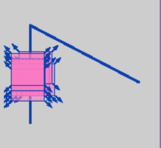
Edge region: no change in edge direction |

Corner region: change in all directions |
The Harris Corner detector calculates a score for each pixel in the image called the corner response which is an indicator of the 'corneryness' of the pixel region. Pixels with high values of corner response correspond to good features.
The basic algorithm is as follows:
- Compute the horizontal and vertical derivatives of the image Ix and Iy by convolving the original image with derivatives of Gaussians
- Compute the images corresponding to the outer products of these gradients.
- Convolve each of these images with a larger Gaussian.
- Compute a scalar interest measure which is an idicator of the 'corneryness' of the feature point.
- Filter bad pixels and report the rest as detected feature points.
Here's how the code would look in Matlab:
            %% 1. Compute the horizontal and vertical derivatives of the image
            % Get x and y gradients of image using gaussian derivative filters of size
            % hsize. This technique is used by Schmid Mohr and Bauckhage (2000) and
            % Triggs (2004)
            [gx, gy] = imgradient(fspecial('gaussian', hsize_grad, sigma_grad));
            % Gradient of Gaussian filtered image is same as filtering image with
            % gradient of gaussian
            Ix = imfilter(image, gx, 'symmetric', 'same', 'conv');
            Iy = imfilter(image, gy, 'symmetric', 'same', 'conv');

            %% 2. Compute the images corresponding to the outer products of these gradients
            %% 3. Convolve each of these images with a larger Gaussian
            blur_filter = fspecial('gaussian', hsize_blur, sigma_blur);
            Wxx = imfilter(Ix.^2, blur_filter, 'symmetric', 'same', 'conv');
            Wxy = imfilter(Ix.*Iy, blur_filter, 'symmetric', 'same', 'conv');
            Wyy = imfilter(Iy.^2, blur_filter, 'symmetric', 'same', 'conv');

            %% 4. Compute a scalar interest measure which is an idicator of the 'corneryness' of the feature point
            Wdet = Wxx.*Wyy - Wxy.^2;
            Wtr = Wxx + Wyy;

            response = Wdet./(Wtr+eps(0.5)); % harmonic mean function given by Brown, Szeliski and Winder (2005)
All that is left to do is to weed out the bad pixels and report the rest as detected feature points. A naive way of doing this would be to
- Sort pixels by their corner response in descending order
- Traverse the sorted pixels from top to bottom
- For each pixel, find the pixels within a radius, and mark these pixels as bad. The radius is a hyperparameter and needs to be tuned for optimum results.
The code for the above, looks as follows:
            % Find corners in Harris response
            corner_threshold = max(response(:)) * thresh;
            harrisim_t = (response > corner_threshold);
            % Get coordinates of candidates
            candidates = find(harrisim_t);  % find nonzero indices
            [r, c] = ind2sub(size(harrisim_t), candidates);
            % Get values of candidates
            candidate_values = response(candidates);
            % Sort candidate values
            [~, index] = sort(candidate_values, 'descend');
            % store allowed point locations in array
            allowed_locations = zeros(size(response));
            allowed_locations(min_dist:end-min_dist,min_dist:end-min_dist) = 1;
            [nr, nc] = size(allowed_locations);
            % select the best points taking min_distance into account
            x = [];
            y = [];
            confidence = [];
            for row = 1:size(index, 1)
                i = index(row);
                if allowed_locations(r(i), c(i)) == 1
                    y = [y; r(i)];
                    x = [x; c(i)];
                    confidence = [confidence; candidates(i)];
                    if ((r(i)-min_dist) > 0) & ((r(i)+min_dist) < nr) & ...
                            ((c(i)-min_dist) > 0) & ((c(i)+min_dist) < nc)
                        allowed_locations((r(i)-min_dist):(r(i)+min_dist),(c(i)-min_dist):(c(i)+min_dist)) = 0;
                    end
                end
            end
            % [x, y] give the location of selected feature points.
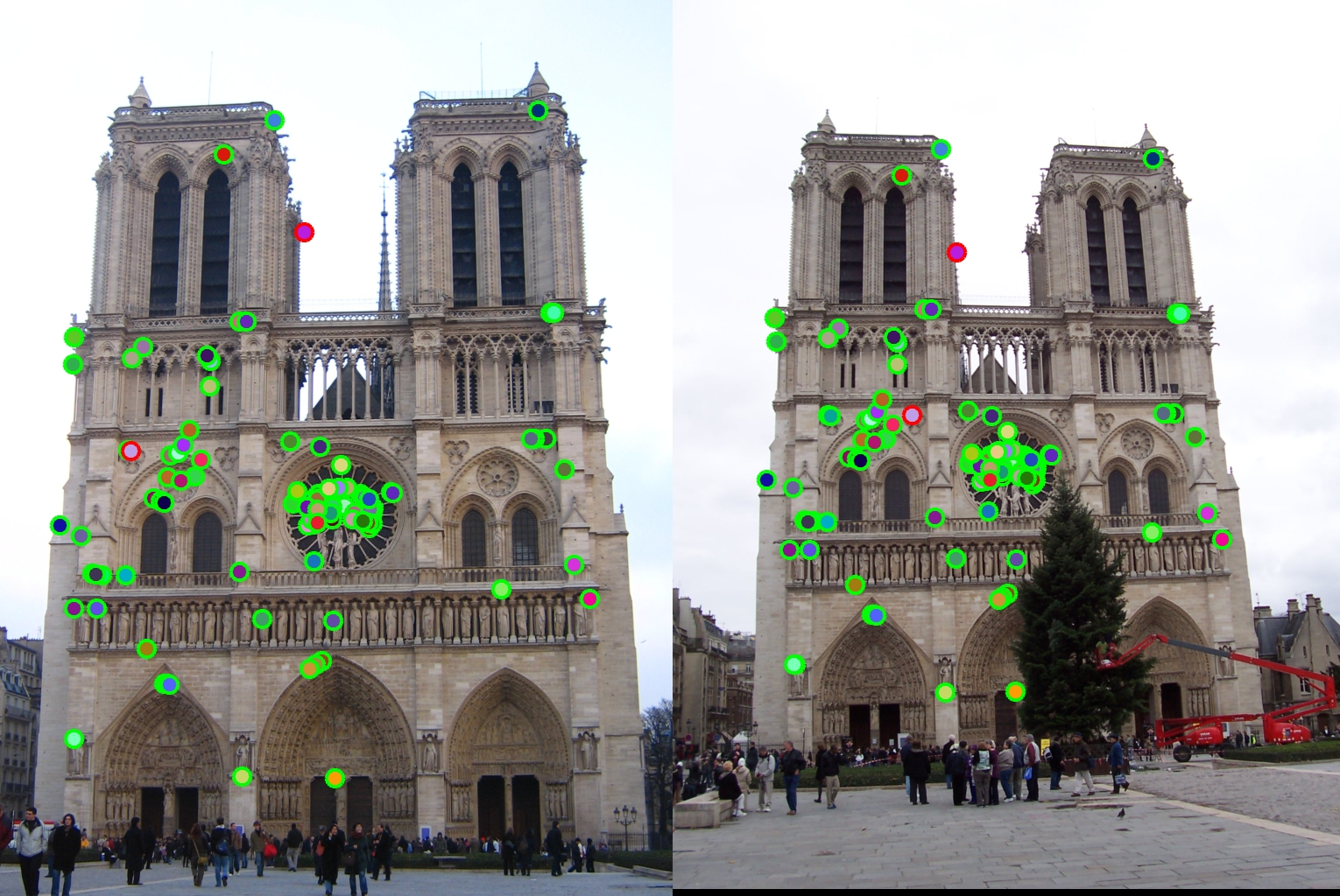
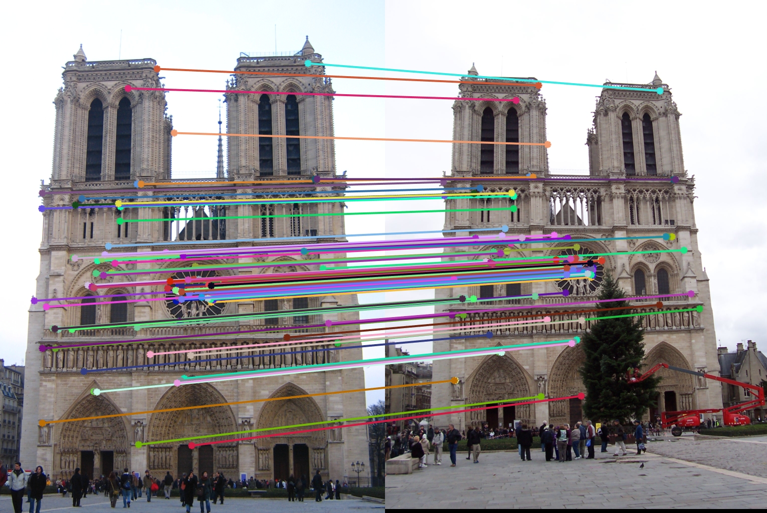
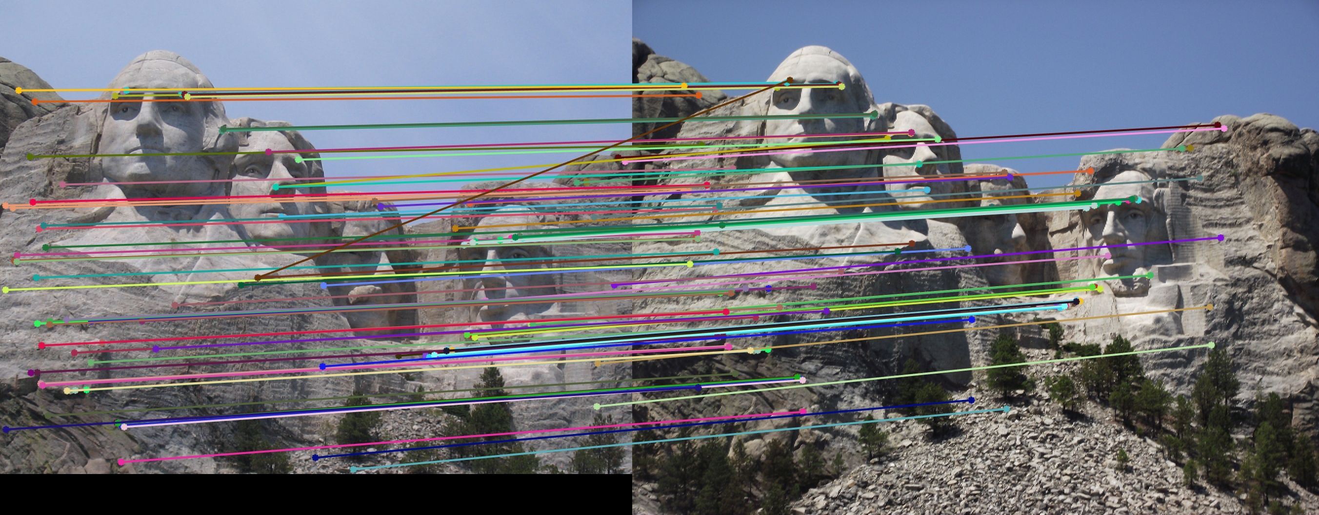
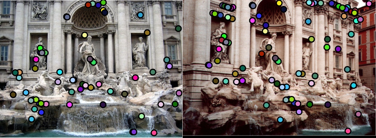
Let's test this out. In the supplied Matlab code, this algorithm can be invoked by passing in the value 'other' to the parameter algorithm in the call to the function get_interest_points in proj2.m. The input image, interest points and matches are as follows:
|
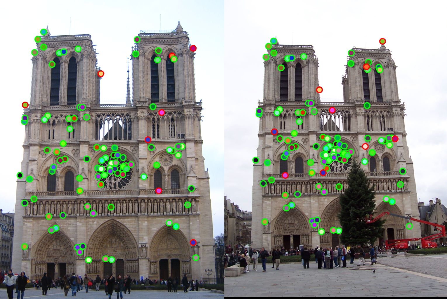
|
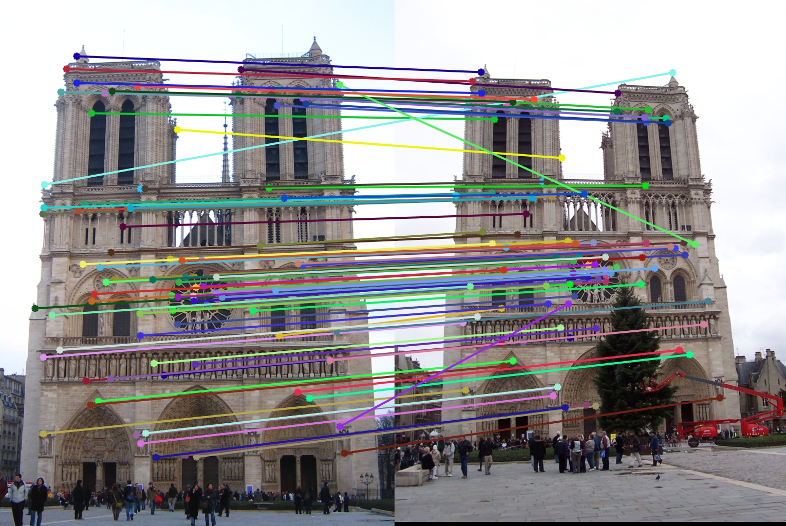
|
The accuracy achieved for this algorithm was 91%. Another way to weed out bad points is to select points that are local maxima in an 8 point neighborhood and are greater than a certain threshold. The code for this looks as follows.
            % Find local maxima which are greater than a threshold
            % Choose top % of values
            sorted_response = sort(response(:), 'descend');
            nms_thresh = sorted_response(floor(0.01*size(sorted_response,1));
            % Find local maxima
            local_max = imregionalmax(response); % returns a binary matrix with 1 at locations of local maxima
            local_max_value = response.*local_max;
            % Find values greater than threshold
            local_max_value(local_max_value < nms_thresh) = 0;
            [y_local, x_local, value_local] = find(local_max_value);
            % Remove corner points
            x_cut = [8 mc-8];
            y_cut = [8 mr-8];
            [x, y, ind] = eliminate_corner_points(x_local, y_local, ...
                x_cut, y_cut);
            confidence = value_local(ind);
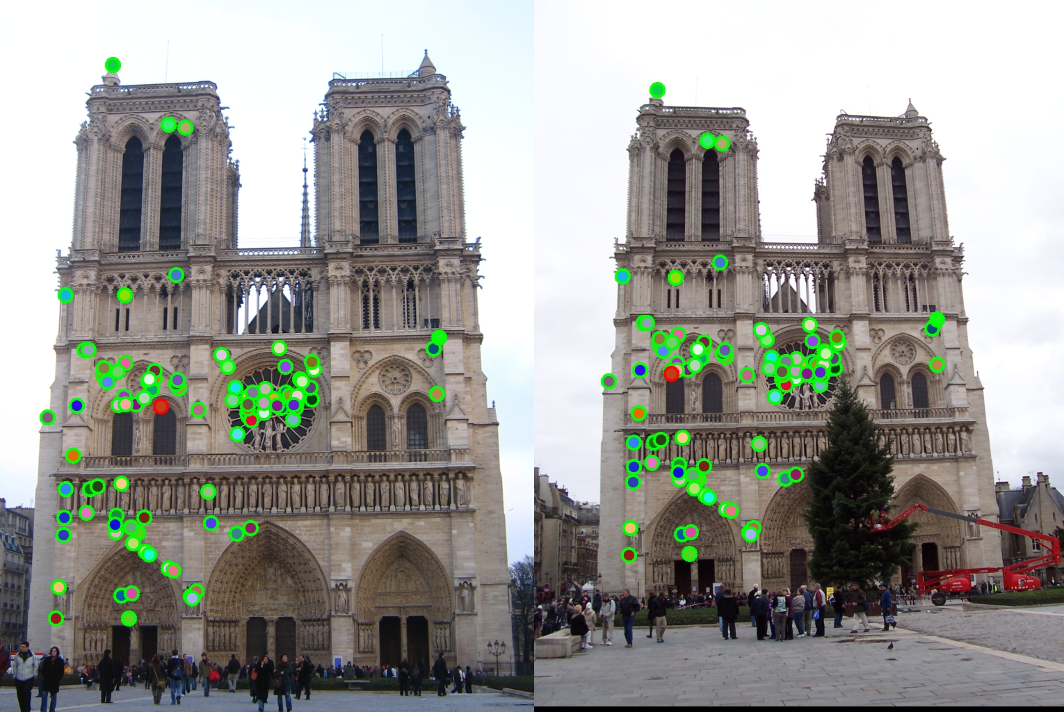
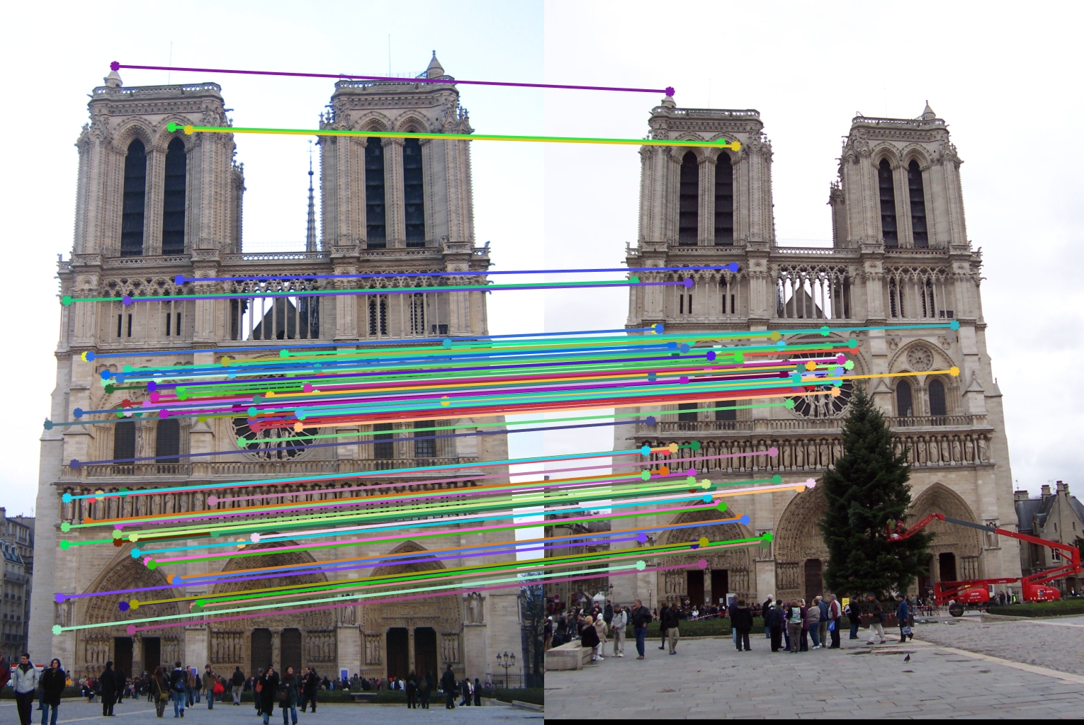
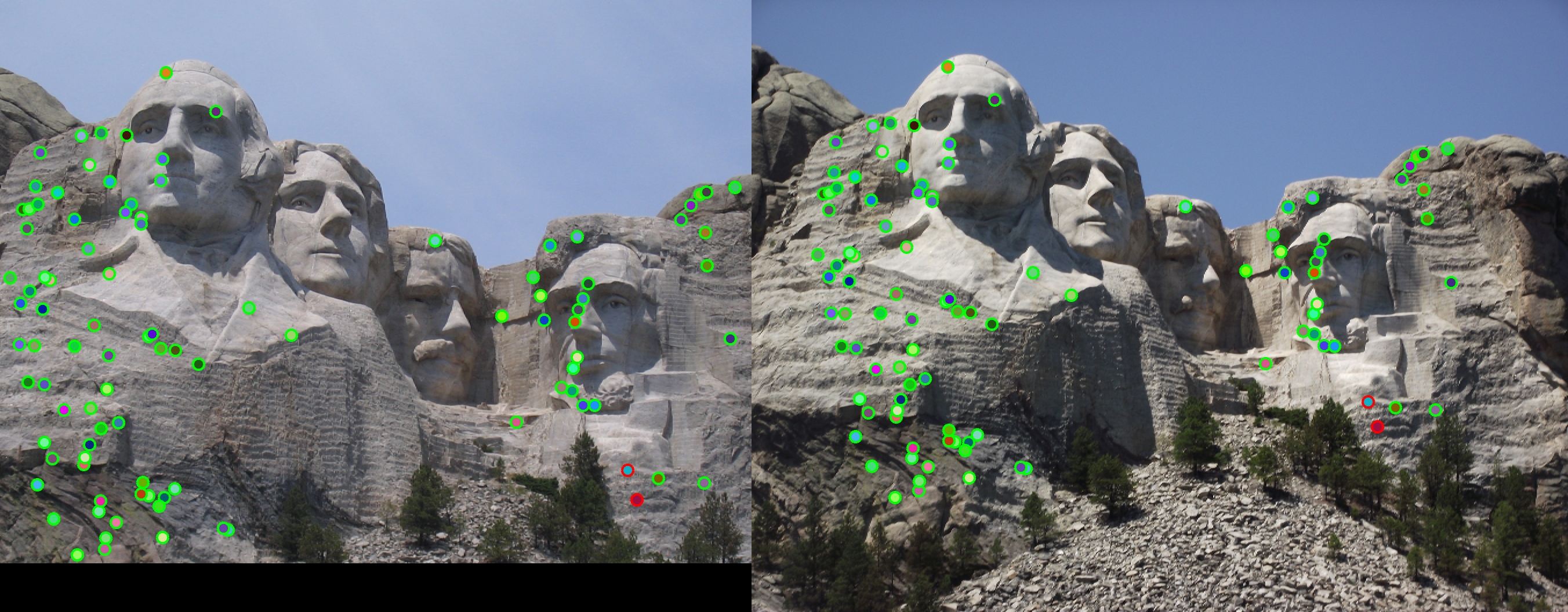
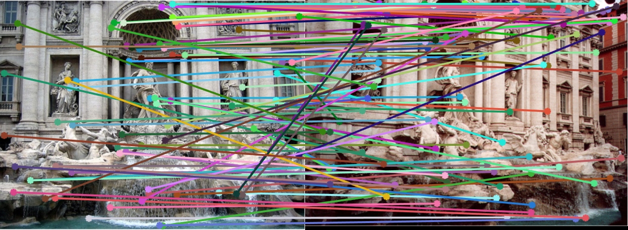
This technique is called non-maximal suppression. Note that the threshold has been set adaptively, instead of being fixed to a particular value. This algorithm can be run by setting the parameter algorithm to 'nms' in the call to the function get_interest_points in proj2.m. Let's test it out. The interest points and matches are as follows:
|
|
The accuracy has now increased to 98%! In some images, nms can still lead this can lead to an uneven distribution of feature points across the image, e.g., points will be denser in regions of higher contrast. An even better way of weeding out bad points is called adaptive non-maximal suppression or ANMS.
Developed by Brown, Szeliski, and Winder (2005), we only detect features that are both local maxima and whose response value is significantly (10%) greater than that of all of its neighbors within a radius r. They devise an efficient way to associate suppression radii with all local maxima by first sorting them by their response strength and then creating a second list sorted by decreasing suppression radius. The code for this algorithm is as follows:
            [m,n] = size(cimg);
            mean_cimg = mean(cimg(:));
            %% Find local maxima
            % Search for the pixels that have a corner strength larger than the pixels
            % around it and larger than the average strength of the image.
            local_max = imregionalmax(cimg);
            local_max_value = cimg.*local_max;
            local_max_value(local_max_value < mean_cimg) = 0;
            [y_local, x_local, value_local] = find(local_max_value);
            % Remove points too close to the border
            [x_local, y_local, ind] = eliminate_corner_points(x_local, y_local, ...
                [border n-border], [border m-border]);
            value_local = value_local(ind);
            num_local_pts = size(ind, 1);
            %% Create uniformly distributed points

            r = zeros(num_local_pts,1);
            for k=1:num_local_pts
                % For each pixel, find other pixels that have a larger score than this
                % pixel
                row_idx = y_local(k);
                col_idx = x_local(k);
                y_ij = y_local(value_local > cimg(row_idx, col_idx));
                x_ij = x_local(value_local > cimg(row_idx, col_idx));

                % Find the nearest pixel with larger score
                if size(y_ij,1)>=3
                    dt = delaunayTriangulation(x_ij,y_ij);
                    [~, r(k)] = nearestNeighbor(dt, [col_idx row_idx]);
                elseif size(y_ij,1)==0
                    r(k) = max(m,n);
                else
                    r(k) = sqrt(max((x_ij-col_idx).^2+(y_ij-row_idx).^2));
                end
            end

            % Sort by radius in decreasing order
            rij = [r, y_local, x_local, value_local];
            rij_sorted = sortrows(rij,-1);

            % Keep the top max_pts number of points as corners
            if max_pts > size(rij_sorted,1)
                max_pts = floor(0.9*size(rij_sorted,1)+1);
            end
            rij_cut = rij_sorted(1:max_pts,:);
            rmax = rij_sorted(max_pts,1);
            y = rij_cut(:, 2);
            x = rij_cut(:, 3);
            confidence = rij_cut(:, 4);
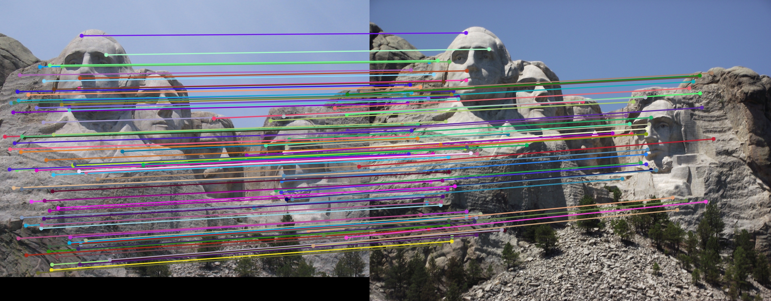
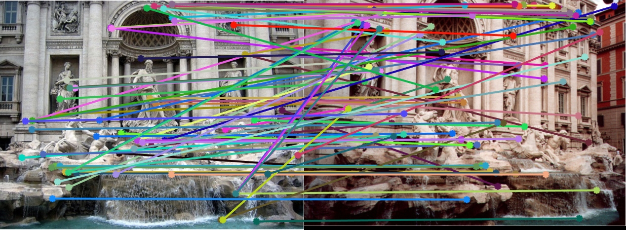
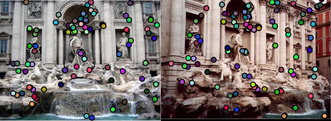
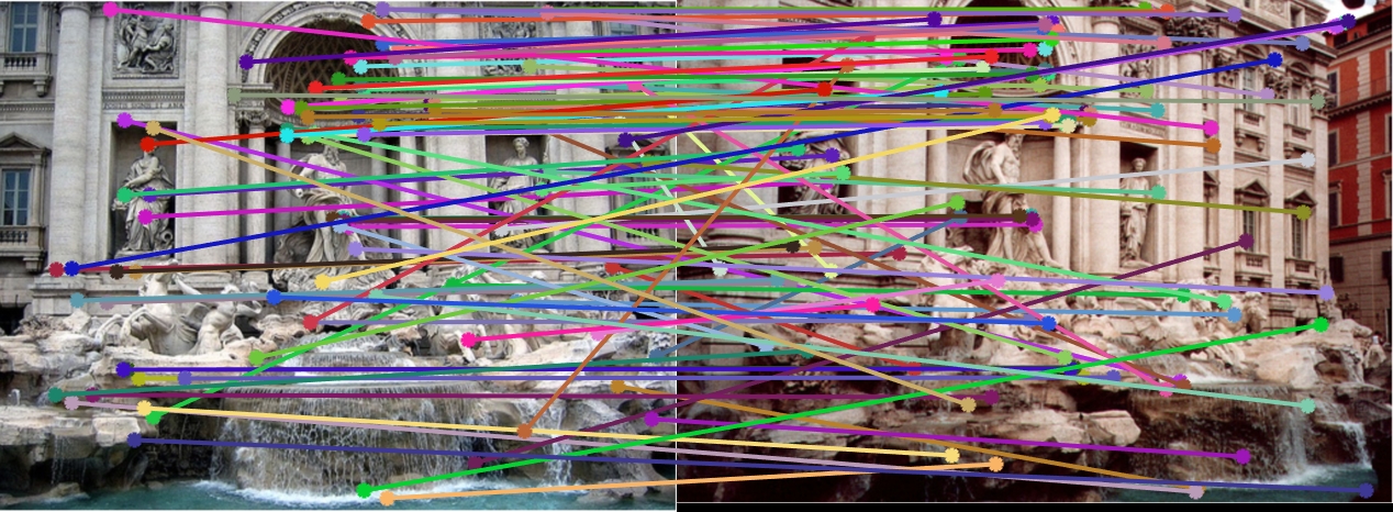
Let's test this out. In the supplied Matlab code, this algorithm can be invoked by passing in the value 'anms' to the parameter algorithm in the call to the function get_interest_points in proj2.m. The interest points and matches are as follows:
|
|
The accuracy is now 99%! That feels good.
2. Feature description
The interest points that we've gotten so far are just that. Point coordinates. It turns out that the patches with these points as centers do not serve as good features. The local appearance of features will change in orientation and scale, and sometimes even undergo affine deformations. Extracting a local scale, orientation, or affine frame estimate and then using this to resample the patch before forming the feature descriptor is thus usually preferable. Even after compensating for these changes, the local appearance of image patches will usually still vary from image to image. How can we make image descriptors more invariant to such changes, while still preserving discriminability between different (non-corresponding) patches? There are a variety of techniques to do this - MOPS, SIFT, LSS etc. I shall describe the Scale Invariant Feature Transform (SIFT) feature descriptor.
The SIFT algorithm is as follows:
- Compute the gradient at each pixel in a 16x16 window around the detected keypoint.
- In each 4x4 quadrant of the window, a gradient orientation histogram is generated.
- The resulting 128 non-negative values form a raw version of the SIFT descriptor vector. To redue the effects of contrast of gain, the vector is normalized to unit length. To further make the descriptor robust to other photometric variations, values are clipped to 0.2 and the resulting vector is once again renormalized to unit length.
The Matlab code is:
            % Extract 16x16 neighborhoods around each index
            features = zeros(1,128);
            hist = @(block_struct) histcounts(block_struct.data, -180:45:180);
            H = fspecial('gaussian', hsize,sigma);
            filt_img = imfilter (image, H,'symmetric','same','conv');
            [~, filt_grad] = imgradient(filt_img, 'sobel');
            for ind = 1:size(x)
                grad = filt_grad((y(ind)-7):(y(ind)+8),(x(ind)-7):(x(ind)+8));
                feat = blockproc(grad,[feature_width/4 feature_width/4], hist);
                feat = feat(:)./norm(feat(:));
                feat(feat>clamp_thresh) = clamp_thresh;
                features(ind,:) = feat./norm(feat);
            end
Scale Invariance
To make the image more robust to scaling, we sample the image at multiple scales, and extract features for each scale. While generating features, we resize the image according the corresponding scale of the feature and generate descriptors. To run this in my code, set the n_scales parameter in the second section of proj2 to some value greater than 1. Using the same threshold value across all scales is going to reduce the accuracy of matching. I have adapted the threshold according to scale in my code.
3. Feature matching
Once we have extracted features and their descriptors from two or more images, the next step is to establish some preliminary feature matches between these images. A matching strategy, determines which correspondences are passed on to the next stage for further processing. There are many matching strategies. A simple one is the Lowe's Ratio Test.
Ratio test
We find the matching descriptors by comparing each feature in image1 to each feature in image2 using Sum of Squared Distance metric. Then for each feature in image1 we select the two features in image2 having less SSD error. And we select one with least squared error, if the ratio of these two features is less than a certain threshold.
A better matching strategy is the nearest neighbor ratio test.
Nearest neighbor ratio test
For each feature, we find the nearest two neighbors in the euclidean space and take their ratio which indicates the confidence of that feature. The features are then sorted according to their confidences and the top n features are taken. This can be done very efficiently in matlab using the knnsearch method.
Results
Here is the application of the above algorithms on various images:
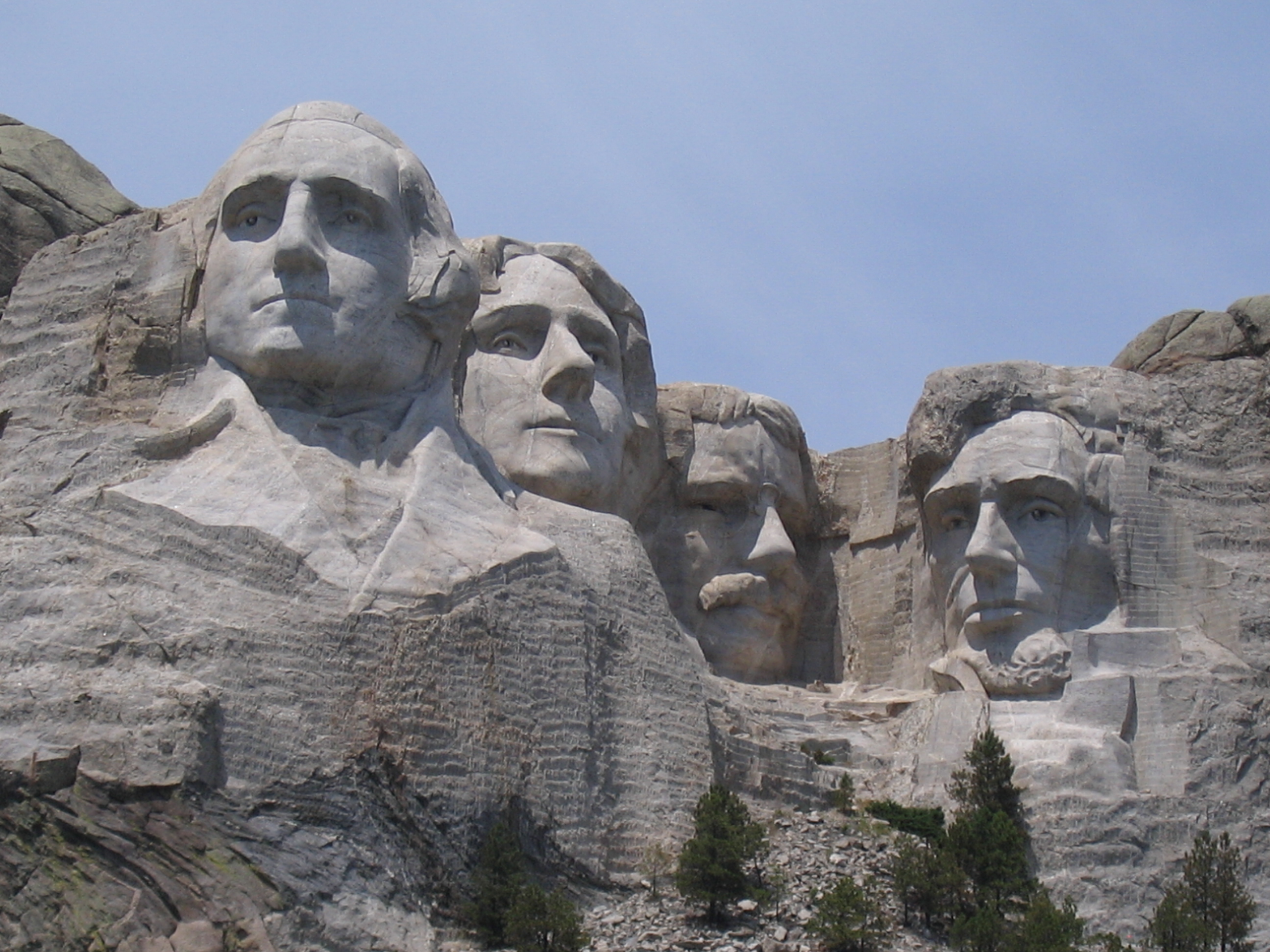
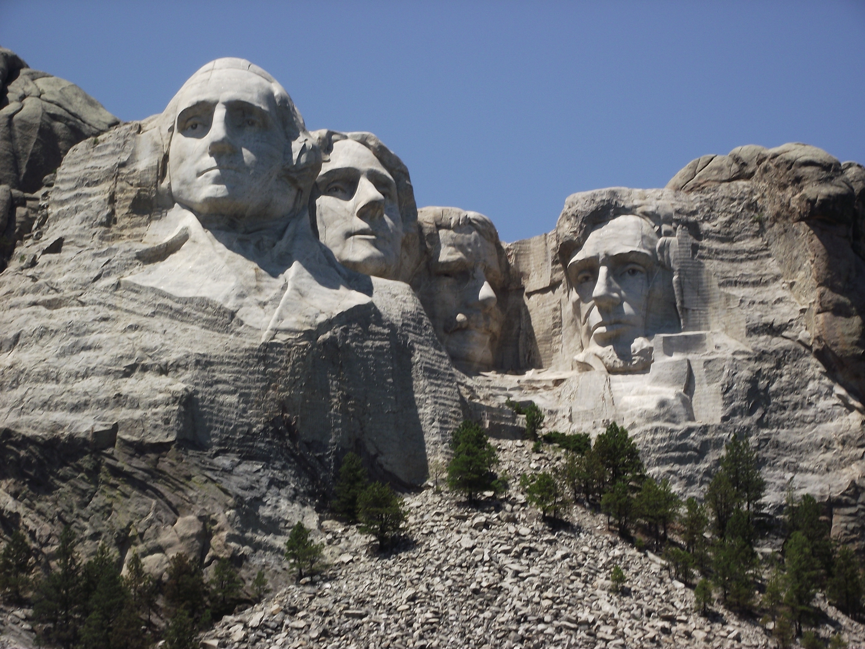
|
Mount Rushmore |
|

|
Naive filtering technique |
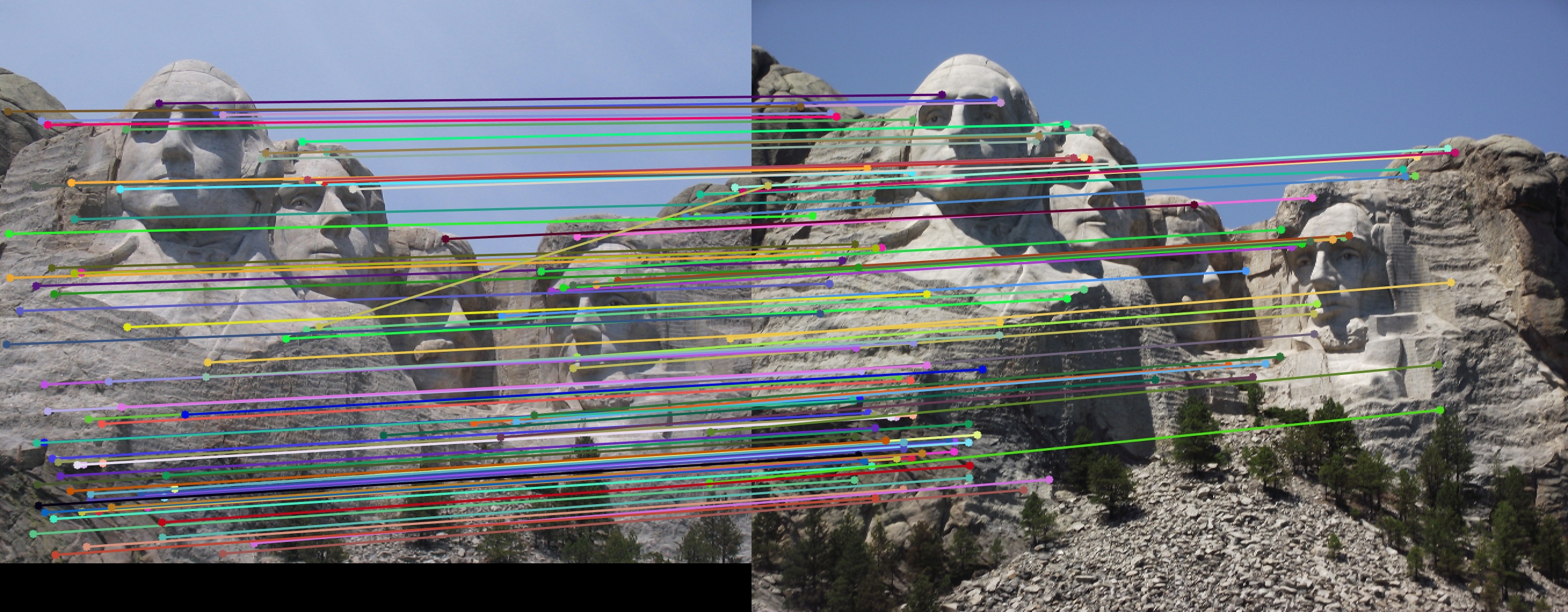
|
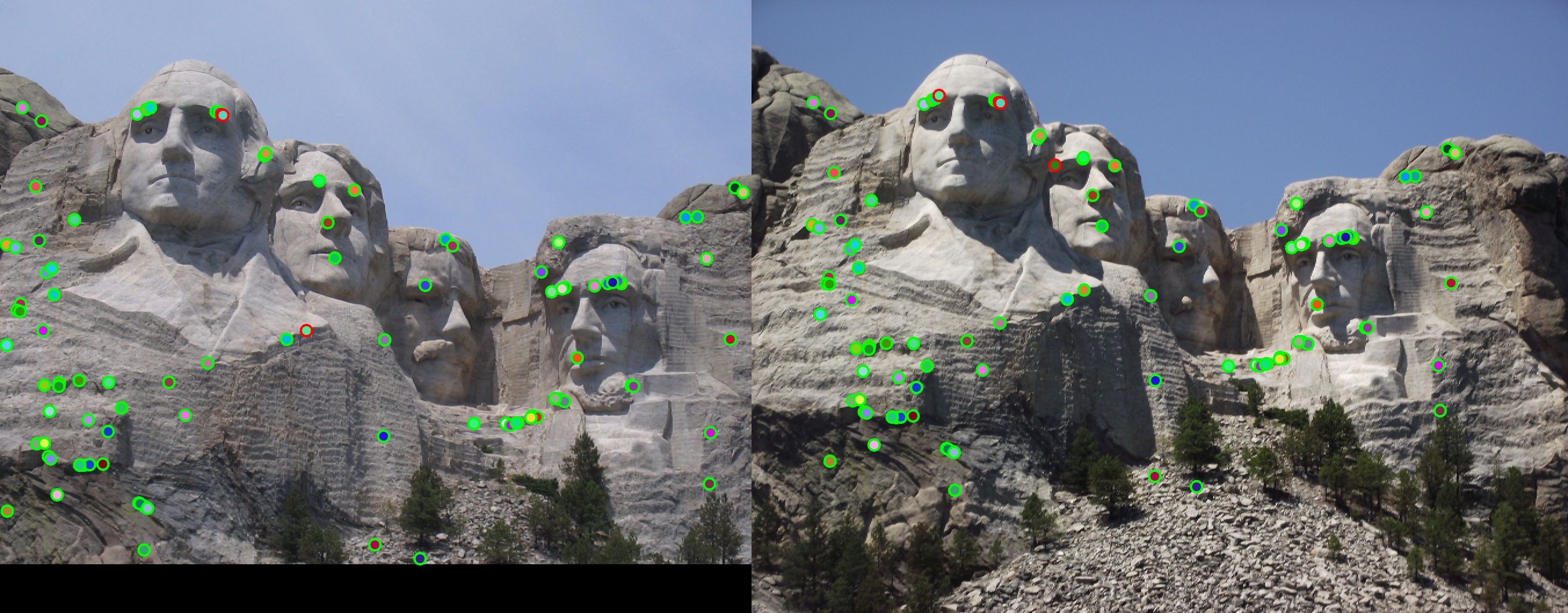
|
NMS filtering technique |
|
|
ANMS filtering technique |
|
|
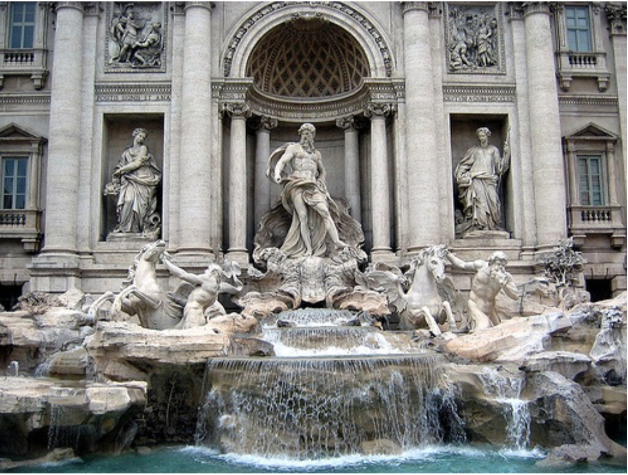
A statue |
|
|
Naive filtering technique |
|
|
|
NMS filtering technique |
|
|
ANMS filtering technique |
|