Computer Vision Project

To implement the SIFT features pipeline, the following were the key steps required.

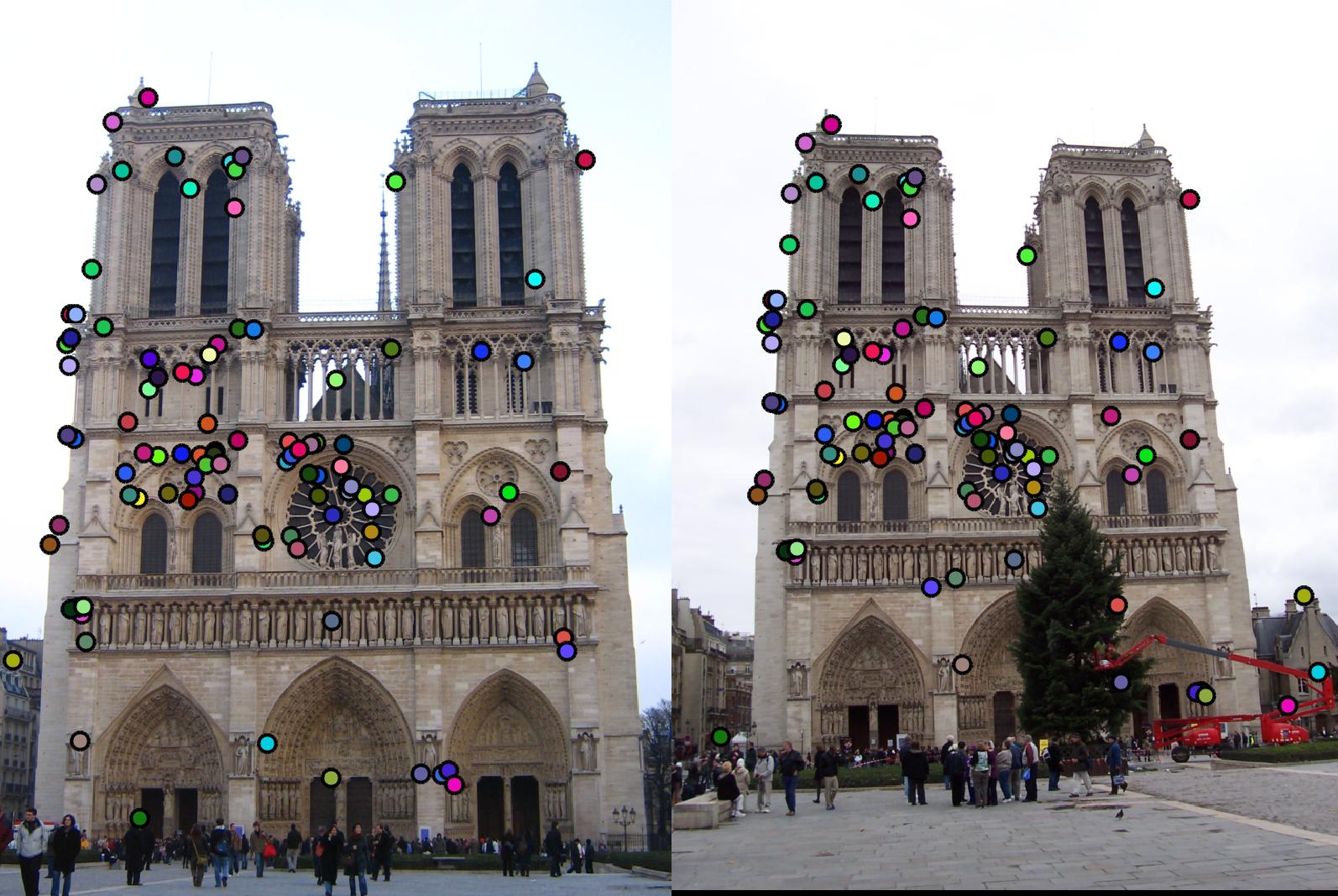
Interest Point Detection

To build an interest point detector, I first took the horizontal(I_x) and vertical(I_y) gradients of the image. In order to evaluate the cornerness function, I convolved the matrix A (as described in Szeleski) with a Gaussian filter as suggested in Szeleski. In order to ensure that the features are spatially distributed, I used local non-max suppression to suppress local minima points and extract as key points only the local maxima. The hyperparameters here were the threshold for the cornerness function and the parameters of the Gaussian filter convolved with the matrix of image gradients.

SIFT Feature Descriptor

The idea here was to take a 16X16 window around each of the keypoints, divide it into patches of 4X4 and compute histograms of the gradient directions for each these 4X4 patches in 8 directions, giving us 4X4X8=128 sized feature vector. While binning, I used bilinear interpolation, i.e., each pixel contributed to two different directions based on the direction of the gradient at that pixel and contributed cos(theta-x) or cos(y-theta) (where x<=theta<y and x,y are consecutive directions in the histogram) into the damped gradient magnitude at that pixel. The gradient magnitude was damped using a gaussian of size 16*16. I also normalized the feature vector and then clamped it to a threshold and then renormalized it as suggested in the code comments.

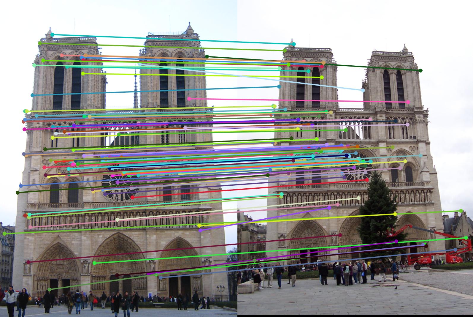
Matching Features

While matching features, I computed the Euclidean distances the feature vectors of image 1 to those of image 2, found matches using the ratio of closest neighbor to the second closest neighbor (confidence). I sorted the matches thus found according to the decreasing confidence and output the top 100 most confident matches.

Results in a table

The implementation required a lot of playing around with hyperparameters. I have selected the best values that I obtained in all cases

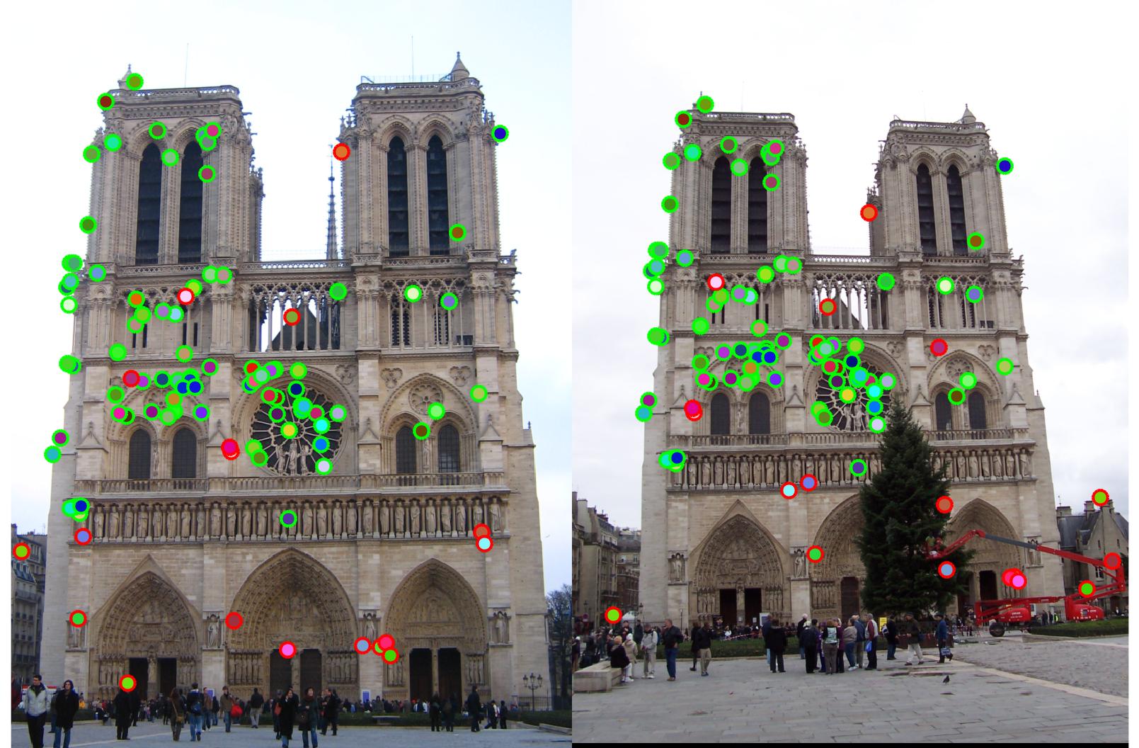
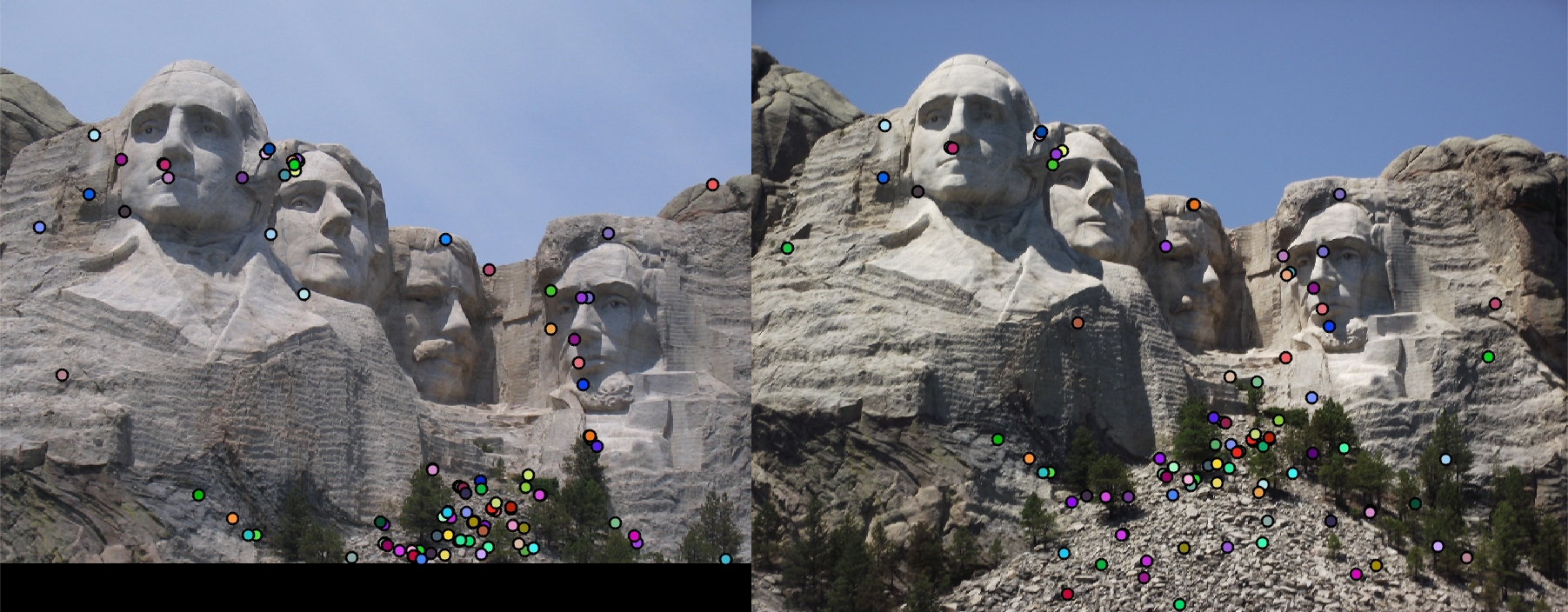
I implemented the pipeline as suggested in the project write up. I first used cheat points to test the accuracy of my SIFT features. I was getting 68% with Notre, 33% with Rushmore and 8% with Gaudi.

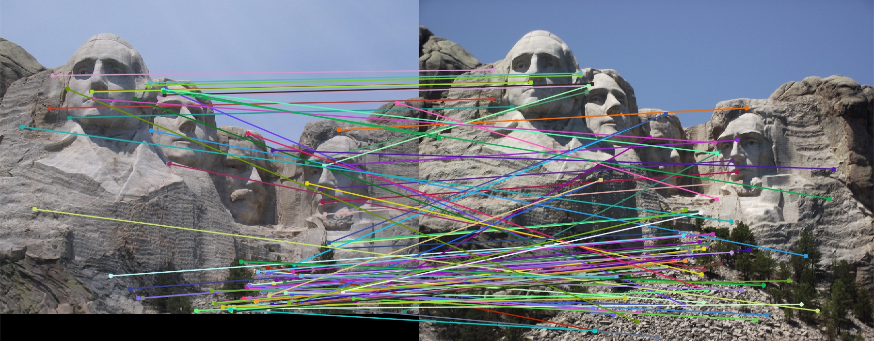
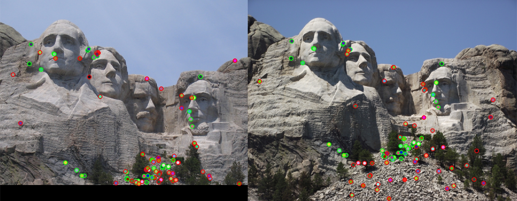
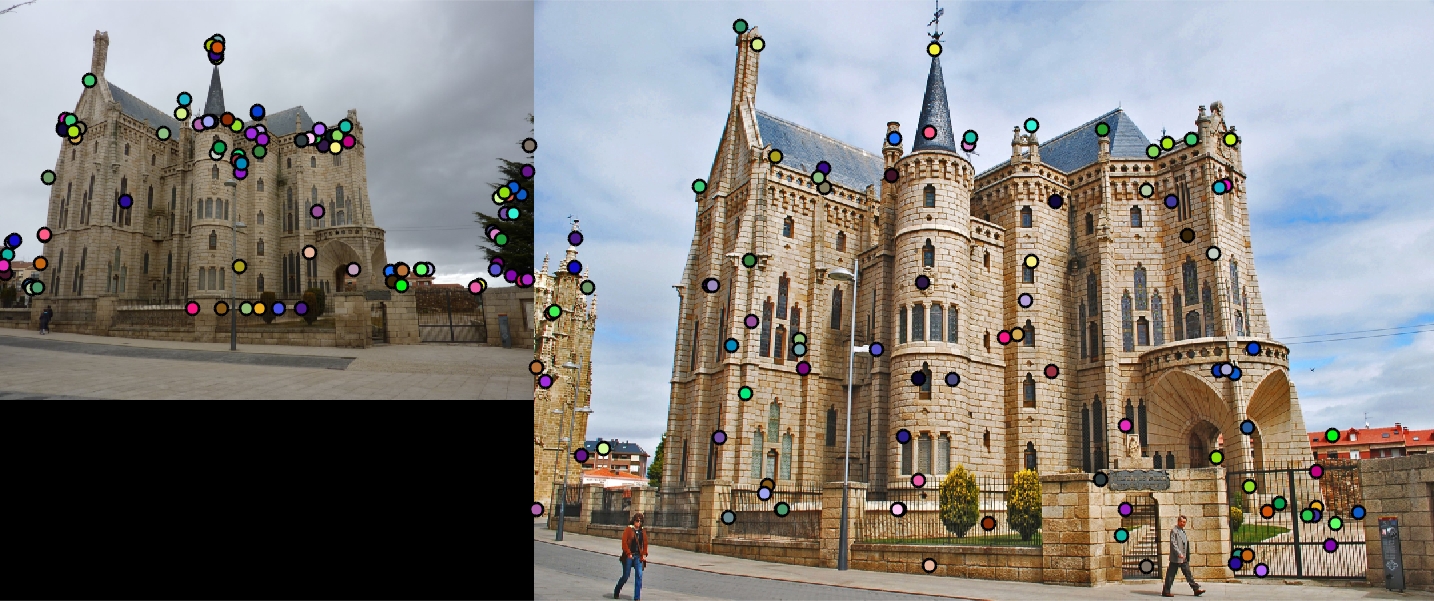
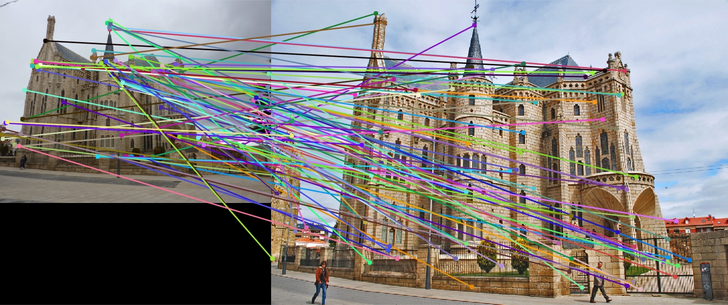
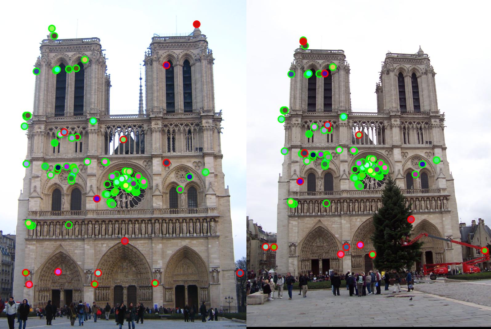
After implementing the entire pipeline I got 89% with Notre Dame, 45% with Mount Rushmore and 2% with Gaudi.

89%

45%

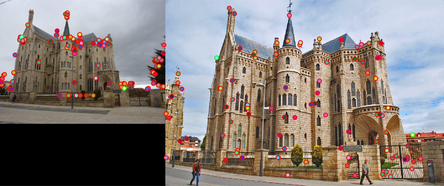
Graduate Credits and Extra Credita

I used kd-tree to reduce the time it takes to find matches. Here are the results for time in seconds. The accuracies remained unchanged

Kd-tree	Non Kd-tree
0.079173	0.360730
0.017458	0.063861
0.123638	1.169924

For extra credits, I implemented PCA to create a lower dimnesional descriptor that gives good enough results. I used 100 images from INRIA holiday data set and computed around 100 feature vectors for each. For all these feature vectores, I computed principal components using svd. All this was done using a new MATLAB script called pca.m and the computed matrix V was saved in the code folder. Here are the results of the accuracy-time(in seconds) trade-off with PCA with 128, 64 and 32 components respectively. The times were computed using kd-tree for matching

Time 128	Accuracy 128	Time 64	Accuracy 64	Time 32	Accuracy 32
0.079173	89%	0.038750	89%	0.015959	88%
0.017458	45%	0.007459	42%	0.005432	38%
0.123638	2%	0.074485	2%	0.031437	3%

Role of hyperparameters

The value of the hyperparameters had a great role in determinig accuracy. I would like to mention some that affected my interest point detection, such as the:

size and variance of the Gasussian filter used to convolve the image,
threshold to the cornerness function,
the size of the sliding window on colfilt used to determine region to select maxima from

I implemented several things in the get_features function to help tweak accuracy:

Bilinear interpolation (increased accuracy by almost 4% on Notre)
Clamping the feature vector to a threshold and renormalizing (increase by 1-2% on Notre)

For the image where I get 89% accuracy, I use a Gaussian of size [3 3] with variance=1, threshold=0.005 and sliding window for non max supression as [8 8]. A few examples of how these parameters affect the accuracy.

With sliding window on colfilt reduced to [3 3] from [8 8]. It leads to selection of more number of redundant points as can be seen in the center circle in the image. Accuracy drops to 82%
With size of Gaussian changed from 3 to 5. Accuracy drops to 86%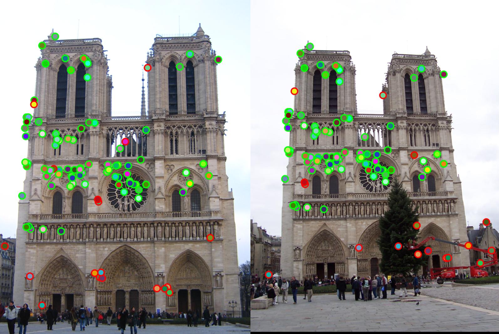
With threshold increased to .01 from .005. Accuracy drops to 79% as fewer good corner points are being detected now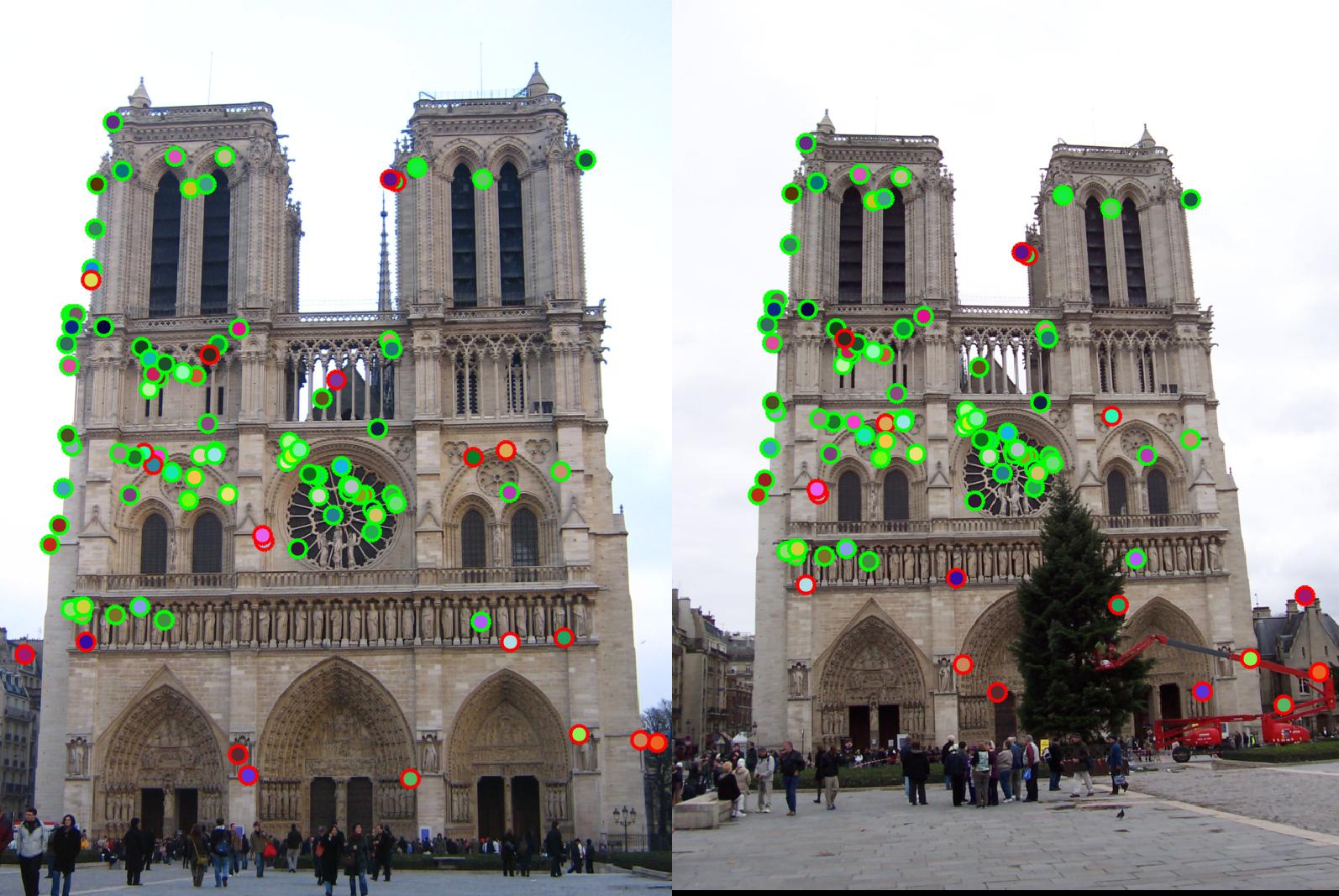