Agrata Kumar

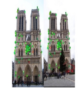
Example of a finding interest points in an image.

Step 1 : Get Interest Points

The first step was to identify the keypoints in the image. There are different techniques of identifying these points in an image, but in this project we used the Harris Corner Detector. A window of pixels was considered around each point in the image. We calculated the corner response function and picked up the points whose surrounding window gave large corner response.

There were a lot of parameters involved in this step which could be tuned to get good results:

1. The window size of the filter used to blur the image and the window size of the filter used for taking the gradient of the image
2. The value of constant alpha
3. The value of the threshold which is used to threshold the corner response.

Local Non Maixmal Suppression

Even after tuning these parameters the interest points were not good, so I peformed the Local Non-Maximal Suppression, to get rid of interest points very close to each other and choosing only the ones with high value of R in a window. We used a sliding window of appropriate size to remove the points very close to each other. As the name suggests, we suppressed the points with local minima in the window and retained only the points with maximum confidence. If we do not get rid of these points then they will cause problems when we match the features, more than 1 point of the first image will be mapped to the same points in the second image, because the distance of both the points in the vicinity will be the same. I used a window of size 5X5 for applying the Maximal Suppression.

Adaptive Non-Maximal Suppression

In the Local Non-Maximal Suppression the window size is fixed. But these points may or may not be spatially distributed. Using the adaptive Non-Maximal suppression the points with the maximum corner strength within the vicinity of the point and with the minimum radius are retained. So the window size around each of the points is different and the track of the value of R and the distance is kept.

Step 2 : Get Features

After finding the key interest points in the image, the next task was to find the feature vectors such that they are highly distinctive. For this we used the SIFT.

SIFT Vector Formation

The image was divided into 16X16 window around each of the interest point and each window was further divided into 4X4 cells. Then the gradient and the magnitude of each of the cell was calculated. The gradient was brought in the range 0-2pi from -pi to pi. Then the range 0 to 2pi was divided into 8 bins. The histogram on the basis of the gradient was calculated and the magnitude corresponding to each value of the gradient was put in the corresponding bin, thus giving us a 128 dimensional vector. This vector is the feature descriptor at the key point.

Step 3 : Match Features

The next step was to match the feature descriptors of the first image with that of the second image.For feature matching I used Lowe's Ratio Test. The Sum of the Squared Distance for each of the feature of Image 1 was caluculated with each of the feature of Image 2. The Ratio of the minimum distance and the second least distance for feature feature was calculated and if this value was less than the value of the specified threshold then the point was retained. The top 100 matched for each of the image were displayed. The lower the value of the threshold the more is the confidence in the matching of the features, the number of correct matches is lowered.

Results in a table

Example 1: Notre Dame

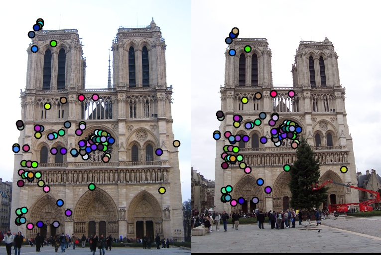
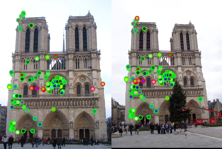
Image 1 showing the keypoints detected in the image with alpha = 0.04 and threshold = 0.0001. Image 2 showing the features detected in the image.

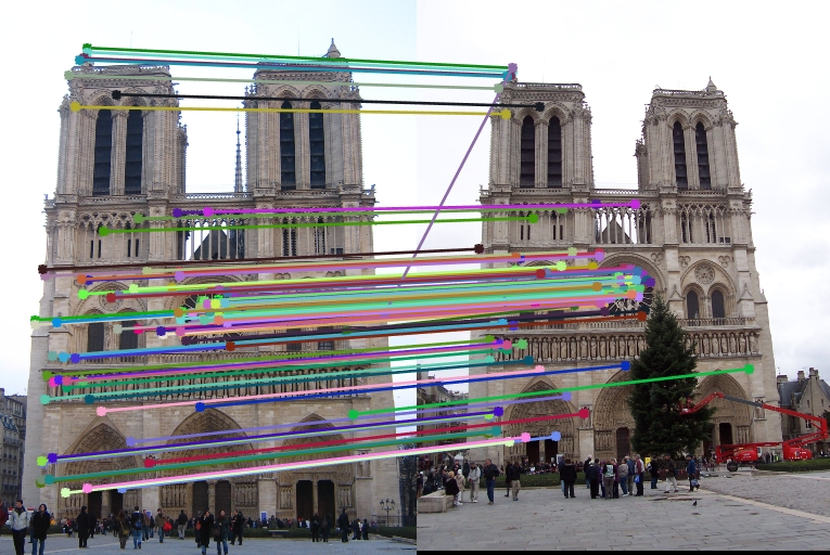
Image showing the matched features in Image 1 and Image 2. 93 features were matched correctly and 7 features were matched incorrectly giving an accuracy of 93%.

Example 2: Mount Rushmore

This although a tricky image but with tuning the parameters, this pair gave good results. The interest points picked up gave good feature descriptors and the feature descriptors match really well, thus showing the appropriate value of the maxima was used.

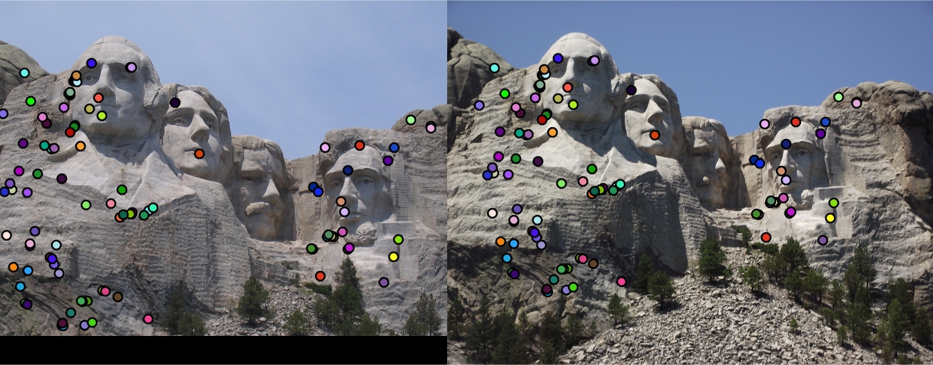
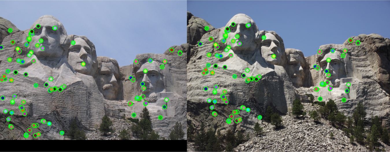
Image 1 showing the keypoints detected in the image with alpha = 0.04 and threshold = 0.0001. Image 2 showing the features detected in the image.

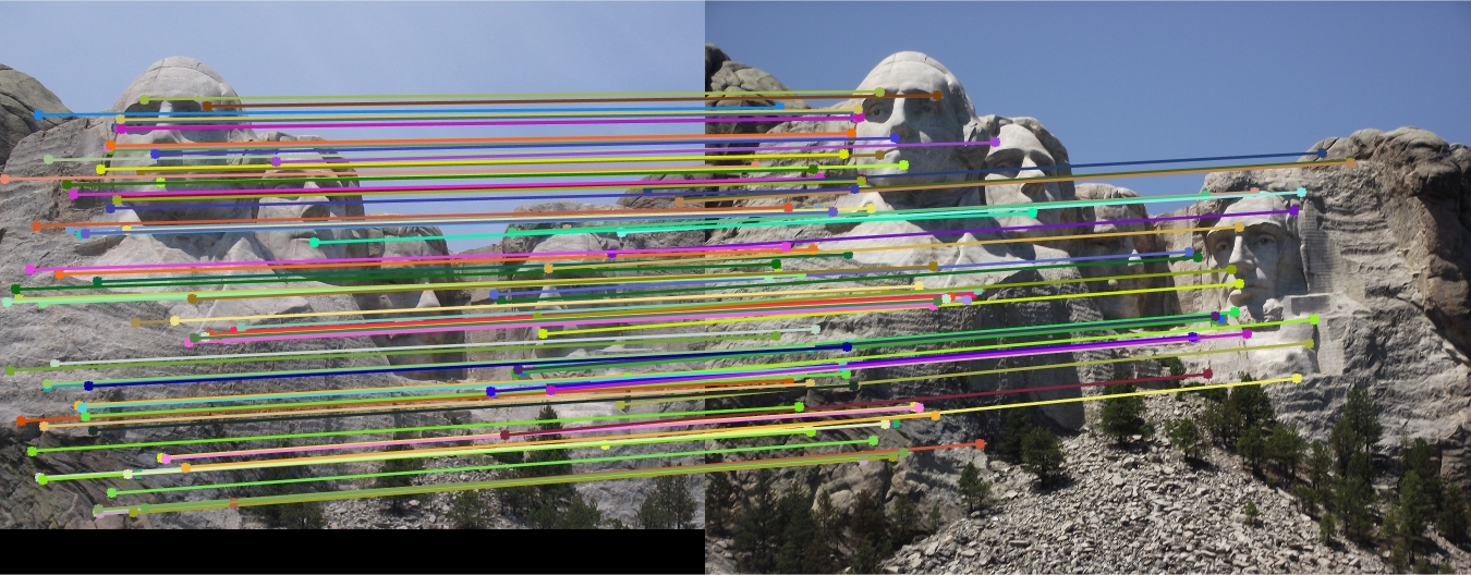
Image showing the matched features in Image 1 and Image 2. 99 features were matched correctly and 1 feature was matched incorrectly giving an accuracy of 99%.

Example 3: Episcopal Gaudi

This is the trickiest pair of images given to us. The number of interest points detected in this pair is usually very small and so the number of matches is equivalently even smaller. Thus, for this pair it becomes even more important to play around with the parameters which we can tune. First, I tried using different filter. If we use just the Gaussian filter then we can get an accuracy of just 10%. So I used a mix of both the Laplacian and Gaussian Filter for this pair. When I tried by creating a histogram with 8 bins then I got an accuracy of about 40%, so I tried changing the number of bins which were there. I reduced the bins from 8 to 4 and voila the accuracy jumped to 60%. But the problem is the number of key points are still 10. As I tried increasing the number of points with same number of bins then the accuracy dropped down to 48% with 25 interest points detected. So I kept the number of bins to 4 for this pair. I further tried changing the cell size from 4X4 to 2X2 and 8X8 but couldnt get better results. The problem with this pair was that the pair of images had different scales.

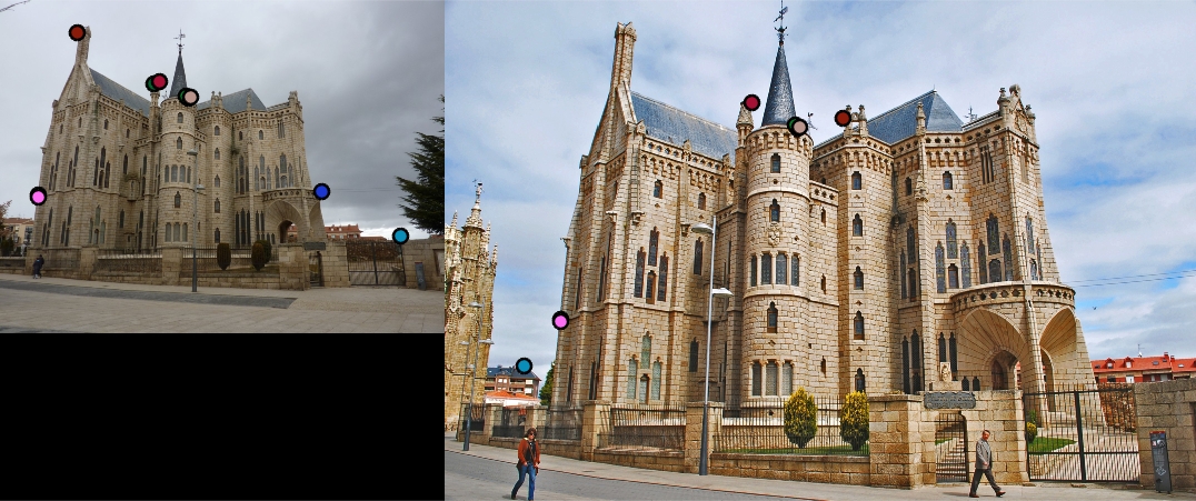
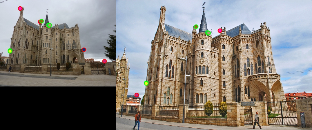
Image 1 showing the keypoints detected in the image with alpha = 0.04 and threshold = 0.0001. Image 2 showing the features detected in the image.

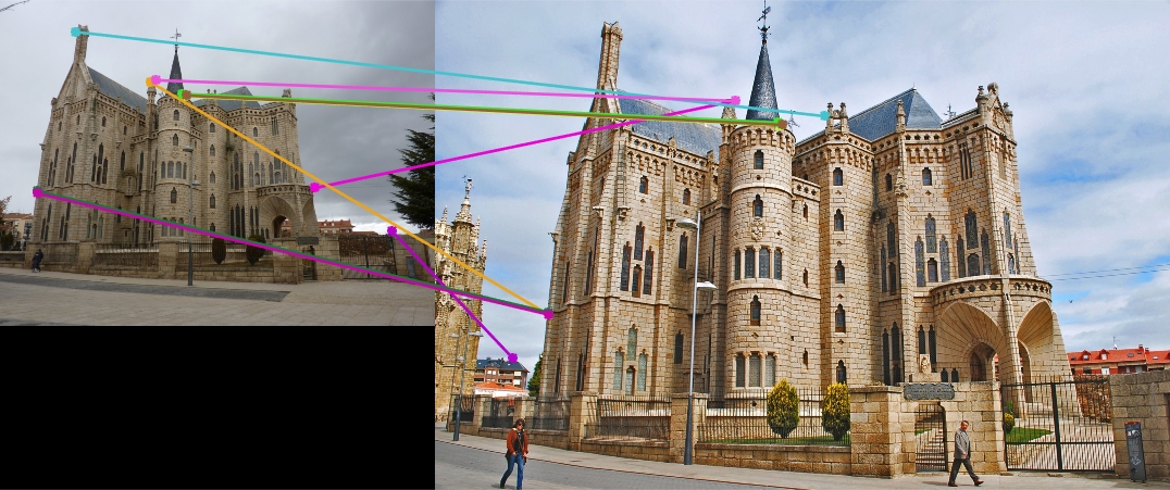
Image showing the matched features in Image 1 and Image 2. 6 features were matched correctly and 4 features were matched incorrectly giving an accuracy of 60%.

Observations

1. Combining Laplacian with the Gaussian Filter while finding the key points in the image can give even better results. The Laplacian filter helps in detecting better points if there is noise in the image (this is what I think might be possible). In our case if we use this combination then we can get an accuracy of about 98% for the Notre Dame image and about 100% in case of Mount Rushmore.
2. Normalizing the features descriptior is important to being all the values to the similar scale as it will further help in matching the features. The results are bad if the features are not scaled properly.
3. We can also use the knn search algorithm while finding the minimum distance while matching features, although it sped up the process of matching the features (it uses the kd tree algorithm, but the results were not so good.

Conclusion

The Local Feature Matching pipeline was developed which gave the key points in the image, gave the feature descriptors for each of the key points and finally matched the feature descriptor of one image with the other.