Ashish Kumar

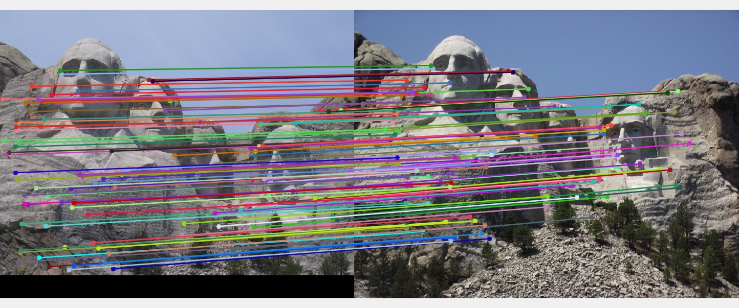
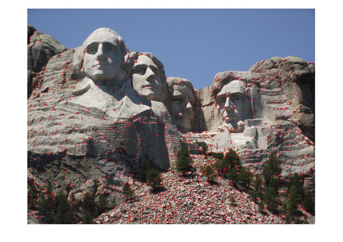
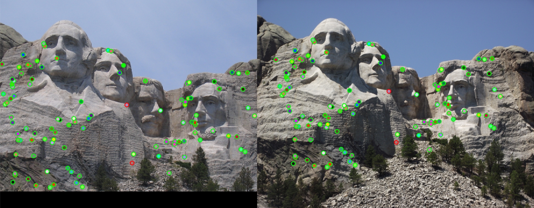
Feature matching of Mount Rushmore

1. Interest Point Detection

1. I apply gaussian filter over the image. The more the smoothing factor, finer the interest points we will get
2. Then I calulcate image gradient and apply gaussian operator over it to find second moment matrix as per Harris Corner Detection algorithm
3. Then I threshold the response matrix and apply non-maximal suppression to avoid getting blobs of inerest points that are closeby. I also ignore the interest points that are situated in the boundary regions make feature descriptors more robust

---

2. Local Feature description

1. I have implemented local feature descriptors based on SIFT
2. The feature descriptor I finally came up with contains 128 elements coming from 16x16 patch centered around the interest point
3. Then I have normalized, clamped to 0.2 and then normalized again the 128 length feature vector

---

3. Feature Matching

1. I have euclidean distance as measure of feature similarity
2. Then I have used the Nearest Neighbour Distance Ratio as best matching feature criteria
3. Then I decide the threshold based on minimum of having either 105 candidates or highest ratio being selected of 0.8

---

Results

Default localmax window: 12x12

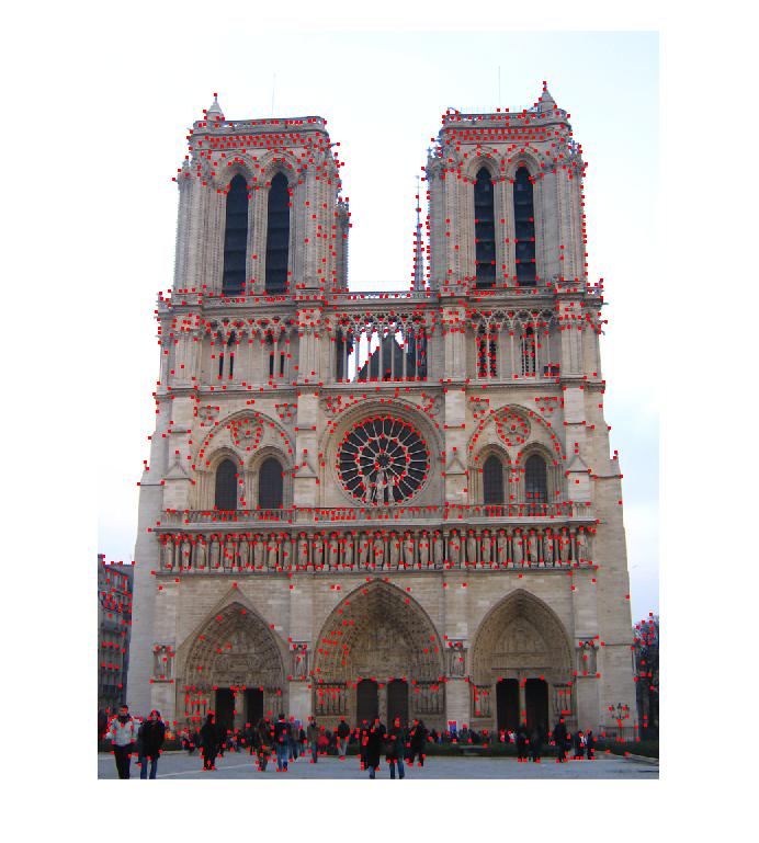
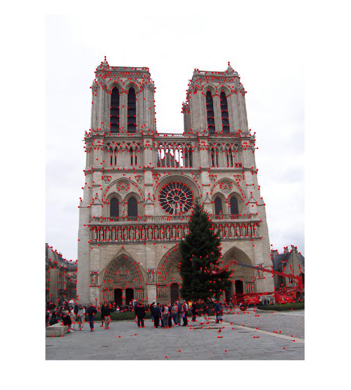
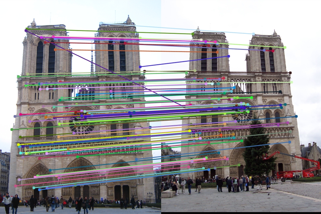
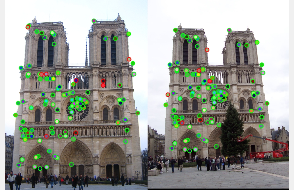
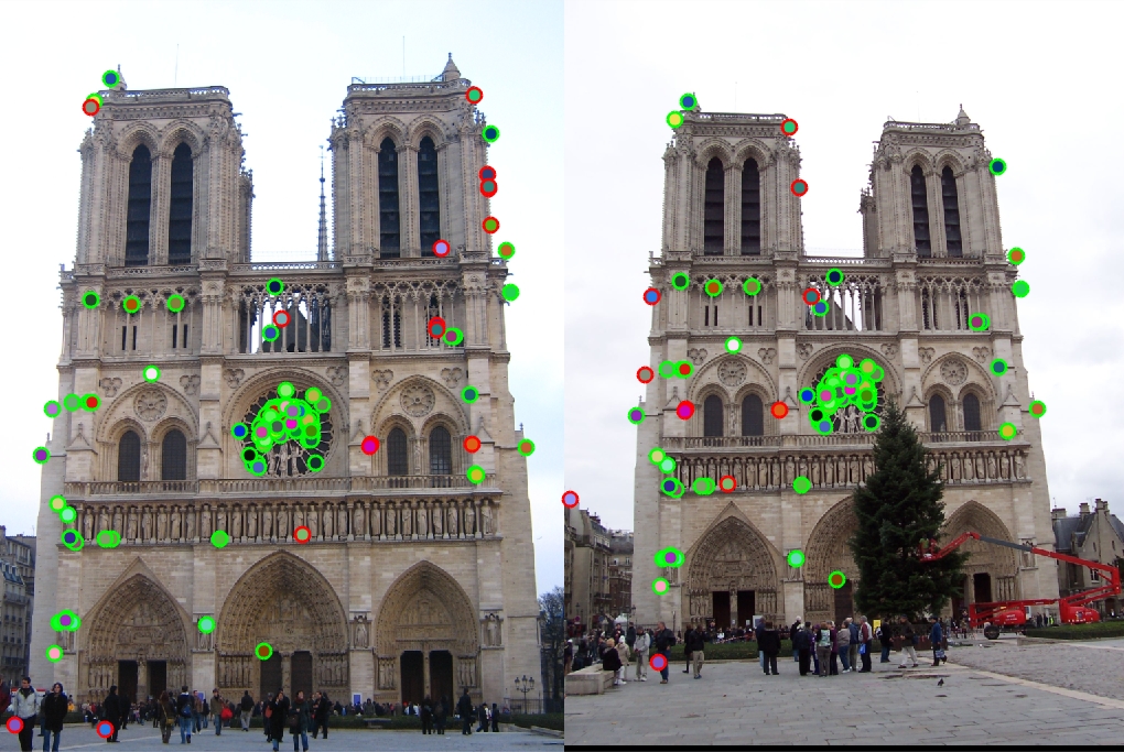
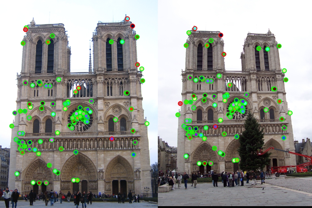
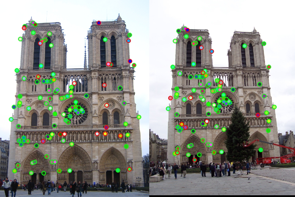
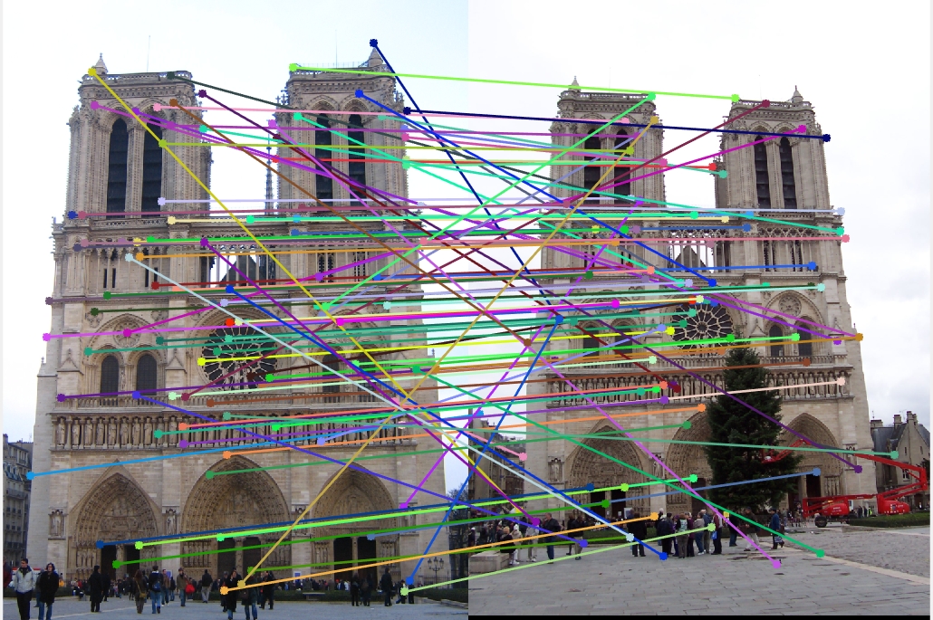
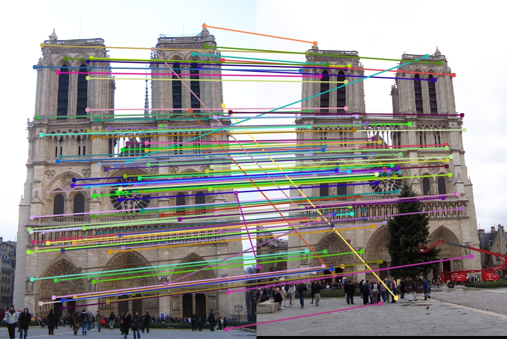
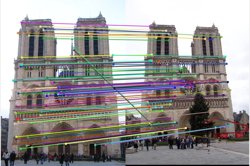
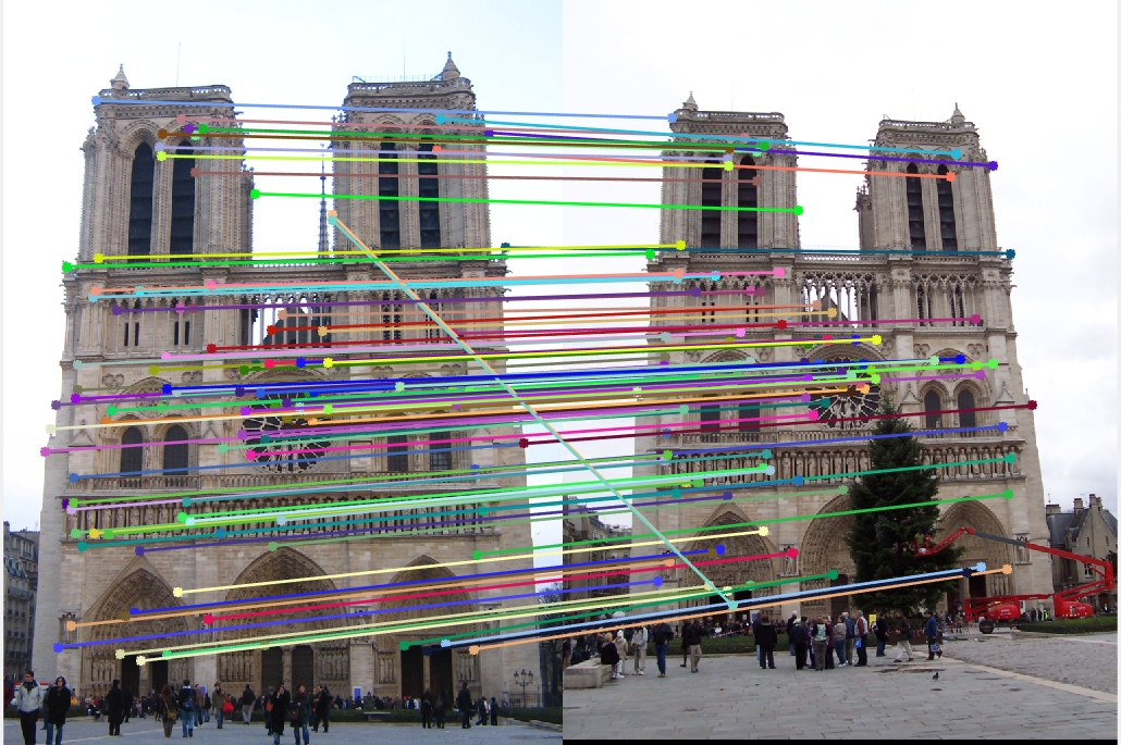
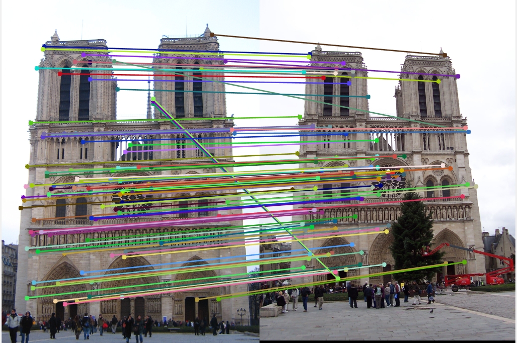
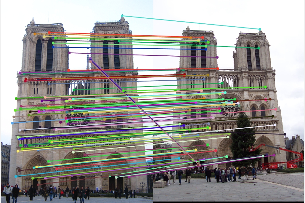
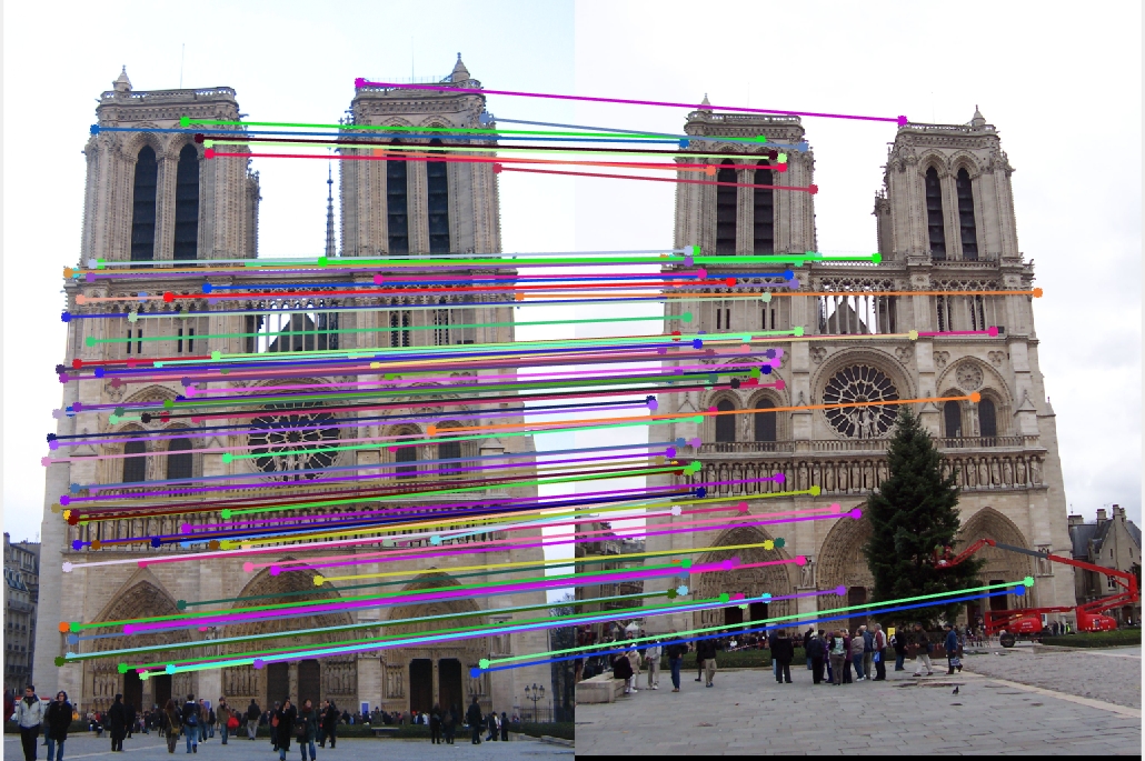
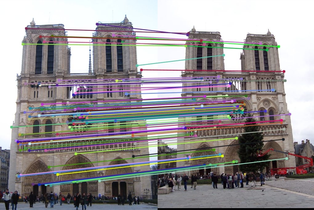
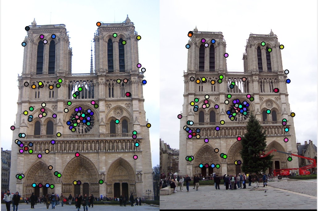
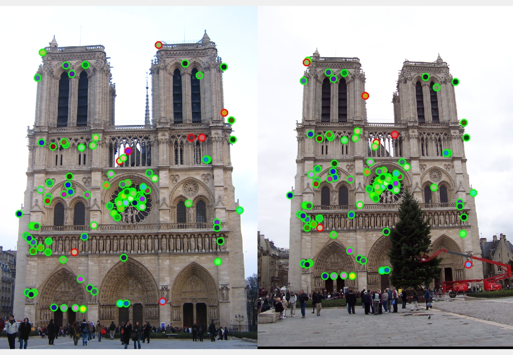
1. Notre Dame(localmax window 8x8): Good Matches = 99, Bad Matches = 6, Accuracy = 94.29%
2. Notre Dame: Good Matches = 96, Bad Matches = 9, Accuracy = 91.43%
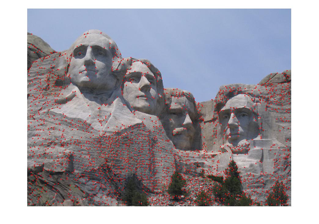
3. Mount Rushmore: Good Matches = 103, Bad Matches = 2, Accuracy = 98.10%
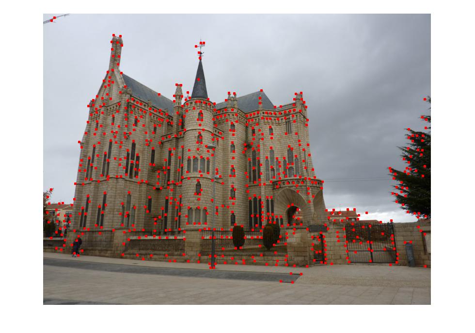
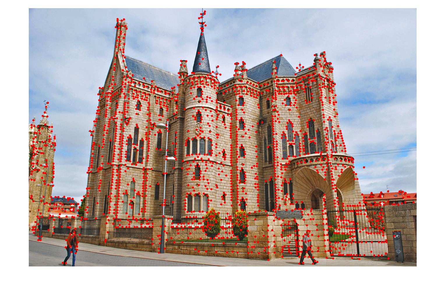
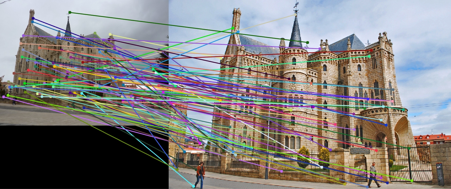
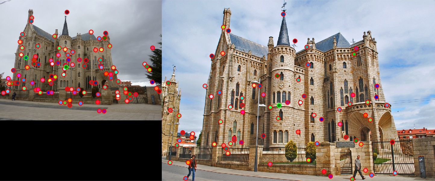
4. Episcopal Gaudi: Good Matches = 2, Bad Matches = 103, Accuracy = 1.90%

As we can see the whole algorithm performed pretty well on NotreDame and Mount Rushmore. But failed miserably on Gaudi. This is mostly due to scaling invariance missing from Harris corner detection method.

---

---

Extra Credits

Interest point detection

1. Adaptive Non-Maximum Suppression

I have implemented an adaptive version of non-maximum suppression to decide dynamically for the threshold. I basically look for 1500 points to reach and keep changing my threshold until I have so many required points. The code is uncommented and can be found in the lower section of get_interest_points.m.

2. Experiment with neighbourhood size in non-max supression

Although local window size at 8 achieved max result for NotreDame but it declined a bit for others. so, I would chose 12 as my default size for better average results

1. Neighbor size 4: Good Matches = 89, Bad Matches = 16, Accuracy = 84.76%
2. Neighbor size 8: Good Matches = 99, Bad Matches = 6, Accuracy = 94.29%
3. Neighbor size 16: Good Matches = 96, Bad Matches = 9, Accuracy = 91.43%
4. Neighbor size 4: Good Matches = 86, Bad Matches = 19, Accuracy = 81.90%

From left to right, then top to bottom: Width: 4, 8 | 12, 16

Local feature descriptor

1. Feature descriptor clamping and normalization

As we can see from below(these stats are for NotreDame), simply normalizing didn't really change the results much, but normalizing, clamping and normalizing again definitely improved the results

1. No changes: Good Matches = 90, Bad Matches = 15, Accuracy = 85.71%
2. Just Normalize: Good Matches = 89, Bad Matches = 16, Accuracy = 84.76%
3. Normalize, clamp at 0.2, normalize: Good Matches = 96, Bad Matches = 9, Accuracy = 91.43%

2. Feature width for feature descriptor

What I found is pretty much in line with different papers citing results on the basis of SIFT descriptor width. As we can see it peaks around 16 and then slowly starts degrading. I also tried at 64 and we can see it drops suddenly due to localization being lost.

1. Width 8: Good Matches = 53, Bad Matches = 52, Accuracy = 50.48%
2. Width 12: Good Matches = 86, Bad Matches = 19, Accuracy = 81.90%
3. Width 16: Good Matches = 96, Bad Matches = 9, Accuracy = 91.43%
4. Width 20: Good Matches = 92, Bad Matches = 13, Accuracy = 87.62%
5. Width 24: Good Matches = 95, Bad Matches = 10, Accuracy = 90.48%
6. Width 28: Good Matches = 94, Bad Matches = 11, Accuracy = 89.52%
7. Width 32: Good Matches = 93, Bad Matches = 12, Accuracy = 88.57%
8. Width 64: Good Matches = 80, Bad Matches = 25, Accuracy = 76.19%

From left to right, then top to bottom: Width: 8, 12 | 16, 20 | 24, 28 | 32, 64

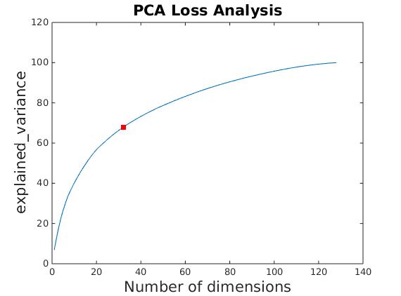
Experiment with Principal Component Analysis to speed up the distance calculation in match features process

• I collected my feature descriptors of length 128 from all the images supplied in extra_data.zip
• The total number of training data was about to be 13453
• At reduced 32 dimension the explained variance ratio for PCA was 67.7%

There was definitely speed up in the matching features process after using reduced dimensions of image features. I was expecting the results to decrease by a considerable margin as the the explained variance was about 67.7% for 32 dimension. Surprisingly the results didn't really degrade at all.

• Without PCA: Good Matches = 99, Bad Matches = 6, Accuracy = 94.29%
• With PCA: Good Matches = 98, Bad Matches = 7, Accuracy = 93.33%

From top to bottom: PCA Analysis, matching features, selected interest points, evaluation