Amritha Ram

Interest Point Detection

This is the first stage of the pipeline, where we calculate the cornerness function using the derivatives of the images and a Gaussian filter. I used the colfilt() function to perform non-maximum suppression, and then found the x and y coordinates of the points I detect as interest points.

The steps I followed were as follows:

1. Find the horizontal and vertical gradients of the image, Ix and Iy, by convolving the original image with derivatives of Gaussians
2. To avoid finding spurious interest points around the edges, suppress the gradients/corners near the boundaries of these images. This is done by just setting their values to 0.
3. Compute the products of derivates at every pixel. From this step we obtain Ixx = Ix.Ix, Iyy = Iy.Iy, and Ixy = Ix.Iy
4. Generate the Harris Corner Response image using the formula : 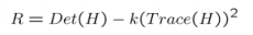where H is the matrix : 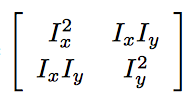and alpha was found to produce good results with a value equal to 0.04.
5. Threshold the response image with some value. The value I used of 1e-3 seemed to work fine.
6. Perform non-max suppression using the colfilt() function, on each sliding window of size 8 to find the max value in the neighborhood. Smaller windows seemed to provide for better accuracy but ended up taking far longer time, so this value seemed to settle the tradeoff the best.
7. Return the local maxima points as interest points.

An observation I made here is that adjusting the threshold on the response image prior to non-max suppression made a great deal of difference to both the accuracy and the speed of the actual process. The reason for this was the number of interest points I eventually ended up with. Finding the right threshold value to give back an optimal number of interest points (for Notre Dame approximately 2500-3000 points) sped up the process quite a bit, while retaining (and in the case of Mount Rushmore, improving) the percentage of accuracy.

Examples of interest points detected:

• Notre Dame example:
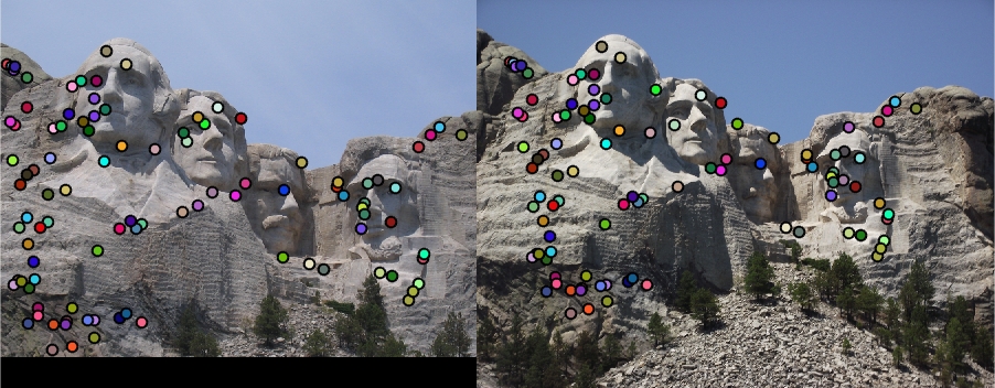
• Mount Rushmore example:
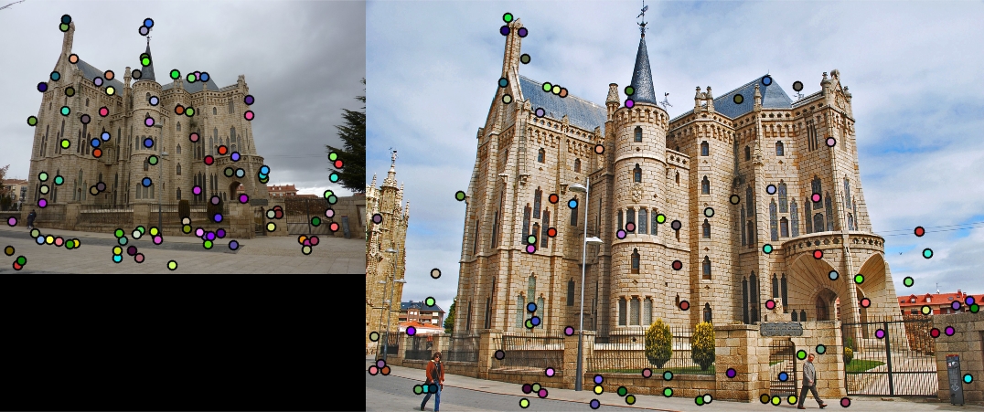
• Episcopal Gaudi example:

Extracting feature descriptors

This is the second stage of the pipleline. Here, we are given the interest points that we detected from stage 1, and try to extract features to match. The steps I followed here were:

1. We first apply the sobel filtered rotated in the directions of the 8 octants onto the image. This gives us the image gradients in the eight orientations we need.
2. For each interest point, we extract a block of feature_width X feature_width size around the interest point from all the eight orientation images.
3. We split this block into a 4x4 cell and within each cell, we find the values of the gradient orientations weighted by magnitude of that direction and do this for all eight orientations to form a histogram of 8 bins.
4. Appending the histograms for all 4x4 windows, we obtain a feature of dimensions 1x128, which we then normalize to unit length.
5. Do this for all interest points so we end up with a number of features.

Code sample for creating feature vector:

feature_matrix = orientedImg(yCord - halfWidth : yCord + halfWidth - 1, xCord - halfWidth : xCord + halfWidth - 1);
cellArr = mat2cell(feature_matrix, [cSize, cSize, cSize, cSize], [cSize, cSize, cSize, cSize]);
for cellRow=1:4
    for cellCol = 1:4
        currCell = cell2mat(cellArr(cellRow,cellCol));
        val = sum(sum(abs(currCell)));
        featureVec(:,index) = val;
        index = index+8;
    end
end

Feature matching

The ratio test : given features from both images, I approached matching the brute-force way, where I found Euclidean distances between all pairs, and then using the closest two matches, I computed a ratio of nearest/second_nearest. The confidence for such a match was the inverse of this ratio. I tried thresholding the matches i.e picking ones under a certain threshold, but found that taking the top 100 most confident matches worked just as well (perhaps even better). Eventually, I sorted the confidences and took out the top 100 confident matches. This approach seemed to yield a good amount of accuracy (92% on the Notre Dame example).

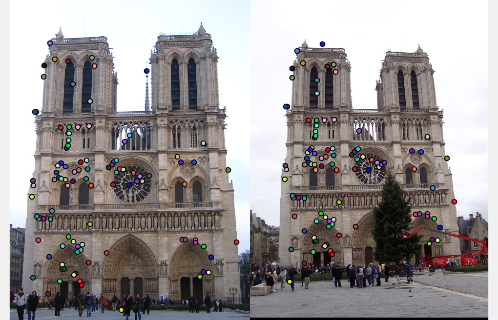
Example results of matching:

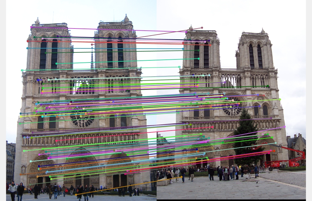
• Notre Dame Example (Accuracy = 92%)
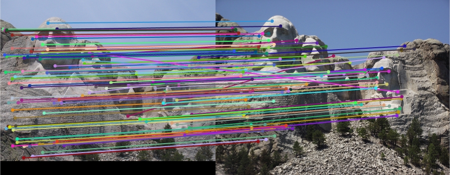
• Mount Rushmore Example (Accuracy = 98%)
• Episcopal Gaudi Example (Accuracy = 8% with sliding window size 6)

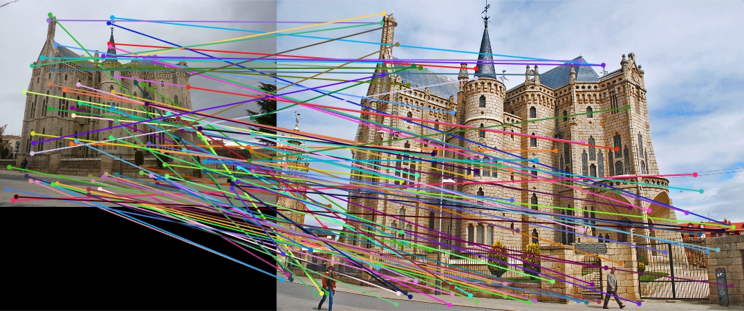
Results of the third example were particularly poorer after implementing get_interest_points. The corner detector seems unable to detect all points of interest well enough to correspond to the ground truth points.

Additionally, to speed up feature matching, I used knnsearch to find the nearest neighbours rather than my earlier brute force distance calculation. This brought down time spent in match_features from 70.925 seconds to 32.635 seconds, which is more than double in speed reduction.

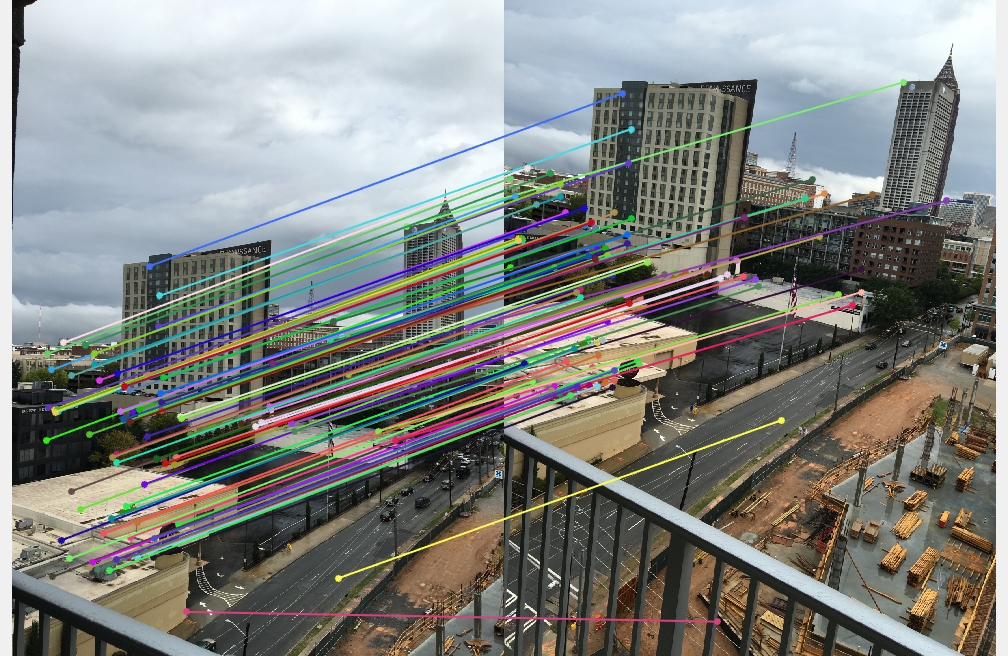
Just for curiosity's sake...

These are images taken from two floors of a high rise building of Midtown Atlanta. I did not have ground truth points to evaluate the correspondence, but just eyeballing the matches seemed to suggest that the algorithm works well on images taken from different angles, though maybe it would not have matched so many points if the images were scaled differently or the angles were too widely varied. Corners detected: 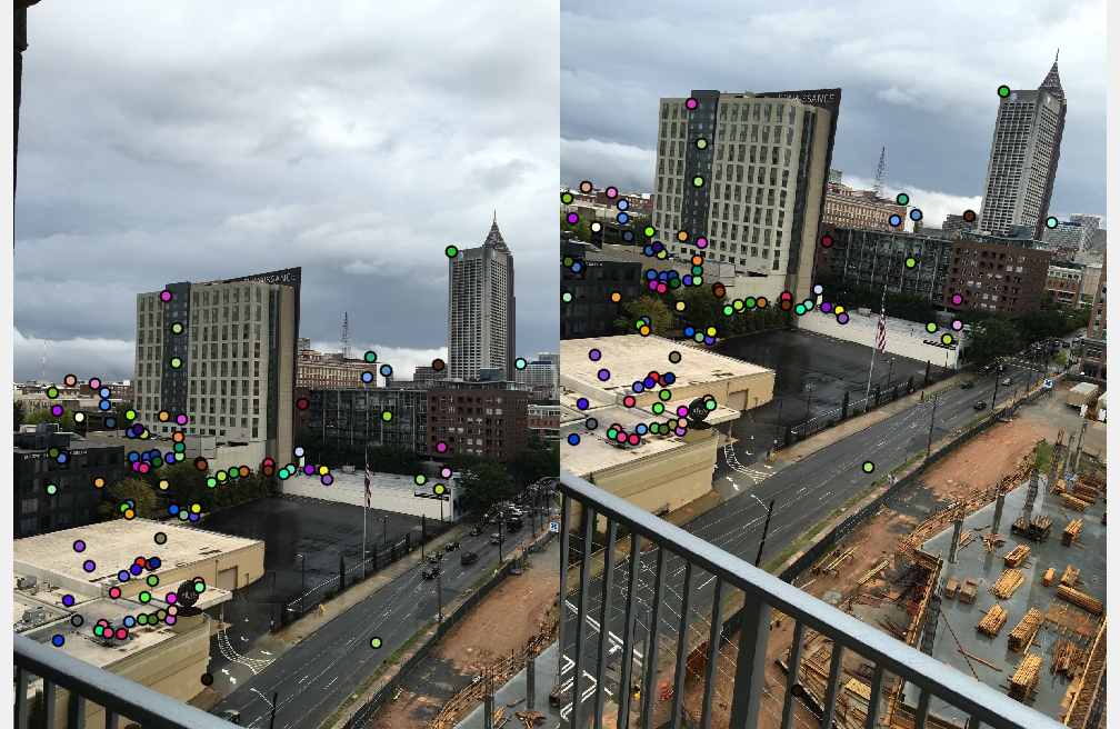Matches: