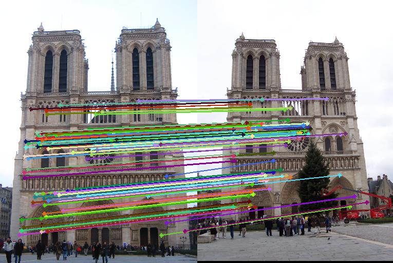
Results of feature matching on the Notre Dame pair.
The objective of this project is to create a local feature matching algorithm to find matching local features in a pair of images. The baseline of this project follows a simplified version of SIFT pipeline, which follow 3 steps:
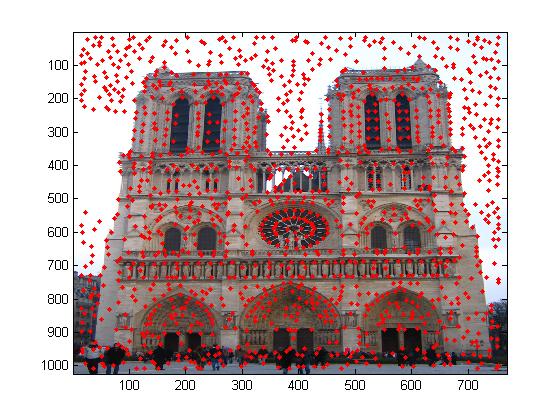
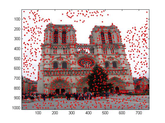
The first step in the local feature matching algorithm is to find distinctive keypoints in the image. The key point detector used here is Harris Corner detector, which is a widely used corner detection algorithm. It is implemented as follows:

Here, a SIFT-like local feature descriptor, as described by David Lowe. After key point detection, we build a local feature around the keypoint that stores information about the gradient magnitude and orientation. The algorithm used is as follows:
Feature Matching was performed using Ratio Test. Here, pairwise distance between the two feature vectors corresponding to the two images was calculated. For each feature, the 2 smallest distances (Two nearest neighbors) are selected and their ratio is computed. If the ratio is below the threshold, then a match between the two images is comsidered, if not, there is no match. Confidence is the inverse of the ratio, and the matches are sorted in descending order of their confidences.
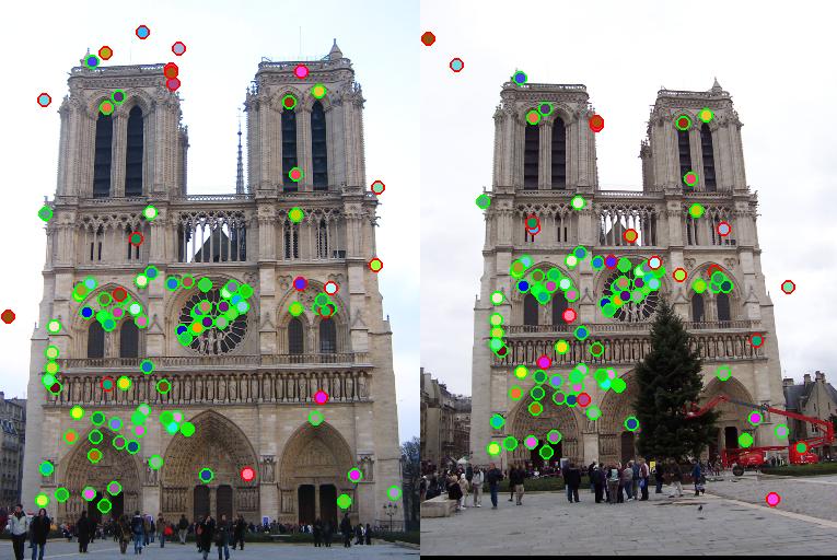
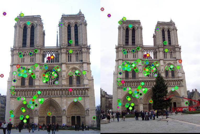
Local feature matching was performed on 2 images depicting the Notre Dame.
Results: Out of the 100 most confident matches, 3 points are matched incorrectly. Therefore, the accuracy here is 97%.
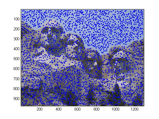
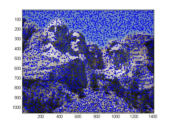
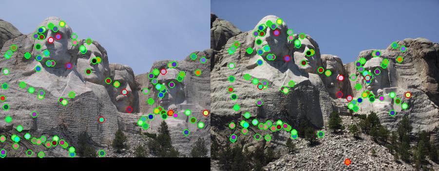
Consider another test case: Two images of Mount Rushmore. The results of feature matching are shown below:
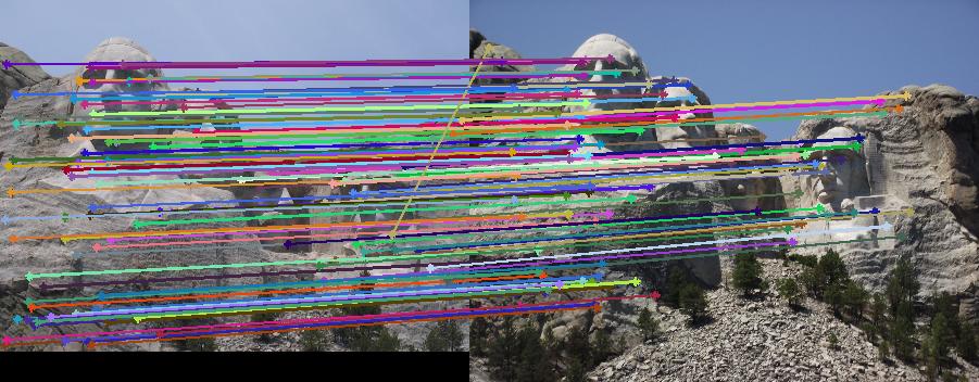
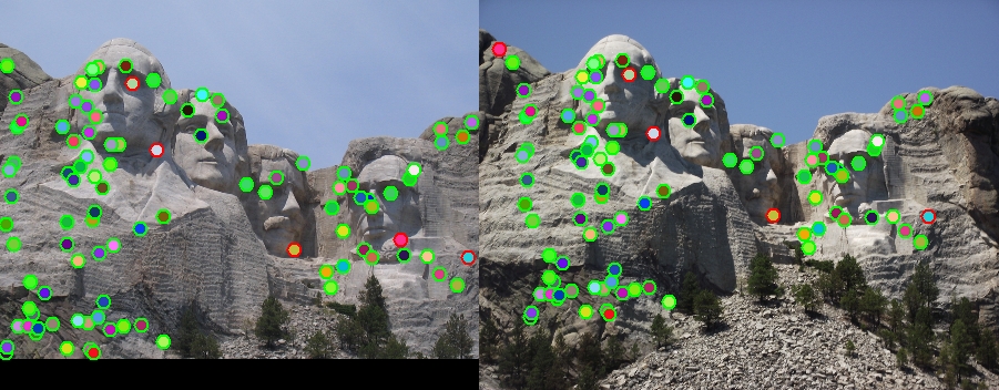
For the Mount Rushmore pair, accuracy is 95%, with 5 points out of the 100 most confident matches matched incorrectly.
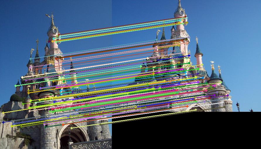
Local feature matching performed on two images of Sleeping Beauty's Castle:
Principal Component Analysis (PCA) is an algorithm that reduces the dimensionality of the data while still retaining as much of the variance in the dataset as possible. The algorithm identifies directions along which the data has maximum variance, called the principal components, which are ordered by dominant dimensions. These principal components can be used to compute new features, of which the first k with the highest variance can be used. This is dimensionality reduction. This works very well with data sets of large dimensions. For example, if the descriptor is 64 dimensions instead of 128, the distance computation would be about 2 times faster, and would require much less memory.
Algorithm:
For each feature:
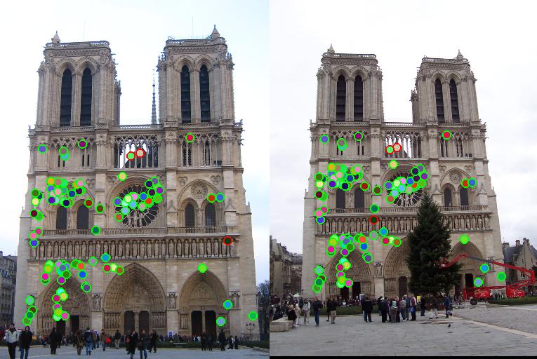
We observe that as dimensionality is reduced from 128 to any value k, accuracy drops, but computational time and memory requirement decreases.
| Image Pair | Accuracy | Accuracy with PCA | |
|---|---|---|---|
| K = 64 | K = 96 | ||
| Notre Dame | 97 | 81 | 94 |
| Mount Rushmore | 95 | 80 | 91 |