Project 2: Local Feature Matching
The general structure of the algorithm I implemented was to first load each image and then find distinctive interst points in each image. I then calculated feature vectors for each interest point. I then used the feature vectors to match the most similar interest points.
Interest Point Detection
I implemented a Harris Corner Detector to find interest points. My implementation first gets the gaussian gradient of the image. I convoluted the Ixy, Ix2, and Iy2 with a larger gaussian gradiant. Then it approximates the harris response by deviding the determinant by the trace. I found the local maximums by comparing each cell with the 8 cells around them from each direction and pick the top 4000 harris corners with the biggest Harris Response.
Calculating Feature Vectors
I implement a SIFT-like feature detector in order to calculate scale-invariant features. In order to do this, I first calculated the gradient of each pixel in the image on a radian scale so I have the direction and magnitude of the derivitive at each pixel. Then for each point which I'm getting the feature vector for, I get grab a square of feature_size(default is 16) which is scaled up and down for differently sized image pairs (by using the ratio of their widths rounded to a multiple of 4). Each of the squares are divided into 4x4 grids. For each grid I calculated a histogram based on the 8 caridinal directions. For each pixel in each grid, I select the 2 buckets in the histogram which are closest to the direction and I chose and linearly interpolate and add the magnitude between the two buckets. I then concatenated all the buckets into a 128 length feature vector. I then normalized the feature vector and square rooted each element in the vector in order to minimize the effect of outliers. I also ran Principal Component Analysis(PCA) on the feature vectors to reduce the 128 length feature vector to a 32 length vector. PCA was run with the features from the 6 project images to create the PCA loadings which was used to calculate the reduced length features.
Matching Features
I matched features by using the ratio test comparing the ratio of the eucledian distance between each point the two closest features. To calculate this, I first used a a kd-tree to run 2-nearest neighbors to find for each point in the first image the 2 closest "feature vectors" in the second image. I used euclidian distance to calculate closeness. I then took the ratio of the euclidian distance between the point and the second closest point and the distance to the closest point. Then I picked the 100 matches with the highest ratios.
Matching Samples
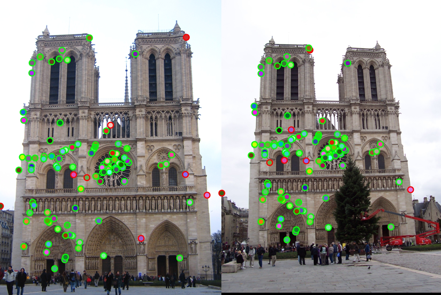
Notre Dame - 92/100 points correctly matched |
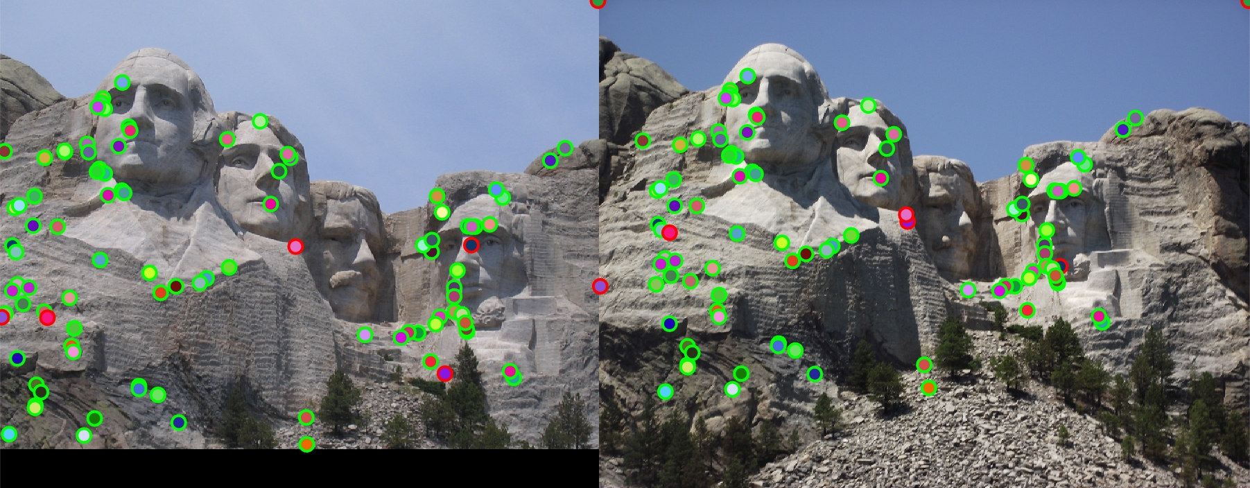
Mount Rushmore - 94/100 points correctly matched |
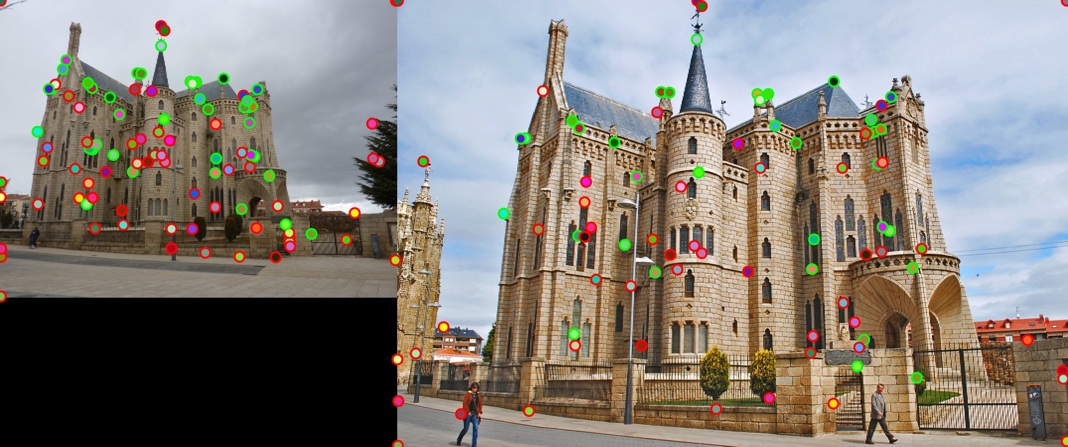
Episcopal Gaudi - 39/100 points correctly matched |
Rotation Invariant Features
I tried testing making the SIFT-like feature detector rotationally invariant but rotating the buckets so that the average bucket with the largest value came first in the feature arrays (I found bucket direction with the highest average by summing up all the buckets in the 4x4 grid). However, this led to slight decreases in matching accuracy in the Notre Dame and Mount Rushmore and large decreases in accuracy in accuracy in Episcopal Gaudi(39% - 26%) so I didn't finish making it invariant by rotating the grid as well. Its likely that the rotational information was being used in matching some of the more difficult feature pairs thus losing the information lowered the accuracy.
Principle Component Analysis
I used Principle Component Analysis to reduce the 128 length vector to a length of 32. I calculated a PCI landing array using features from the each of the two pictures of Notre Dame, Mount Rushmore, and Episcopal Gaudi and chose the 32 most significant resultant features from PCI. Below are the results of using the reduced feature set.
| Photo | Original Runtime for Feature Matching | Original Matching Accuracy | Runtime with Principle Components | Matching Accuracy with Principle Components |
|---|---|---|---|---|
| Notre Dame | 1.508699 seconds | 91% Accuracy | 0.278784 seconds | 92% Accuracy |
| Mount Rushmore | 2.632817 seconds | 95% accuracy | 0.935214 seconds | 94% Accuracy |
| Episcopal Gaudi | 1.262764 Seconds | 43% Accuracy | 0.210863 Seconds | 39% Accuracy |
In these timings, I included the time of multiplying the features by the PCA landing matrix to get the smaller features. The smaller feature set significanly lowered the computation time for matching by as much as 80% while having not too significant impacts on the accuracy. In fact it raised the accuracy on the Notre Dame set and only lowered Mount Rushmore by 1% and Episcopal Gaudi by 4%.
Using KD-tree for Matching
I also implemented using a KD-tree for matching using the Matlab knnsearch function. Unfortunately, when compared to the exhaustive knnsearch implementation, the KD-tree actually usually performed slower than the exhaustive search, as much as 50% slower (around 0.15 seconds). This is likely due to the still relatively large size of the feature set being unsuitable for their implementation and a rather optimized exhaustive search method.