Anh Tuan Van, GTID 902530344

Trying to relate a dot in each image.

Accuracy of dots.

1. Project Intro
2. Code
3. Results
4. Conclusion

Code

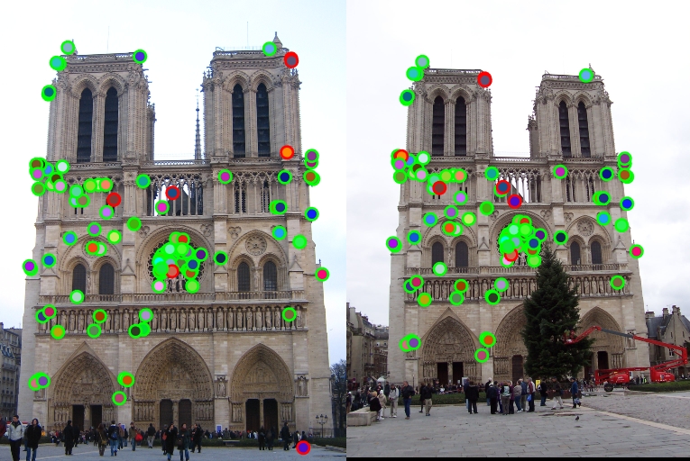
Point detection

This is described in Szeliski 4.1. A major part of this project is interest point detection, also known as key points detection. Shifted images is apt to provide large changes in intesity, helping to find key points. The first step is to filter the image with derivated guassian filters, in order to get the values needed to get the Harris value. This deals with editing the get_interest_points.m file. The small Gaussian filter is then convolved with a larger Gaussian, which would get the variables needed for the harris detection formula.

	[Gx,Gy] = gradient(fspecial('gaussian',[3, 3], 0.5));

	gx = imfilter(image,Gx);
	gy = imfilter(image,Gy);

	gxx = imfilter(gx,Gx);
	gxy = imfilter(gy,Gx);
	gyy = imfilter(gy,Gy);

	Ixx = imfilter(gxx,fspecial('gaussian',[16 16],2));
	Ixy = imfilter(gxy,fspecial('gaussian',[16 16],2));
	Iyy = imfilter(gyy,fspecial('gaussian',[16 16],2));

The following satisfies the following variables in the harris formula:

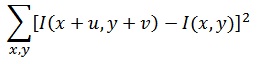
From there, we create the response matrix, which analyzes the 'cornerness' of each point given an intensity change. That code is demonstrated here, along with the application of the harris fomula:

	responseMatrix = (Ixx.*Iyy)-Ixy.^2-0.06.*(Ixx+Iyy).^2;
	responseMatrix(1 : 10, :) = 0;
	responseMatrix(end - 10 : end, :) = 0;
	responseMatrix(:, 1 : 10) = 0;
	responseMatrix(:, end - 10 : end) = 0;

The following code shows the response sorting of the response matrix.

	% sorting the responses to get the best keypoints
	index = imregionalmax(responseMatrix);
	sortedResp = sort(responseMatrix(index),'descend');
	keyPoints = 1000;
	topResp = sortedResp(1:keyPoints);
	x=[];y=[];
	for aPoint = 1:keyPoints
	    [row,col]=find(responseMatrix==topResp(aPoint));
	    x=[x; col];
	    y=[y; row];
	end

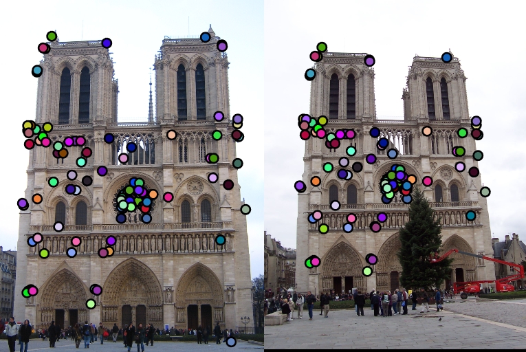
Feature description

The SIFT pipeline next builds local feature descriptors. First, we divide up a 16x16 grid around each point. We then comput the gradient histogram with a gaussian filter. We sum up the magnitudes according to orientation, and then do some normalization to make it easy to process by Matlab. This is done in Szeliski 4.1.2.

	% Creating the guassian filters
	gaussian = fspecial('gaussian', [feature_width, feature_width], 1);
	convolvedGauss = fspecial('gaussian', [feature_width, feature_width], feature_width / 2);
	[GaussDx, GaussDy] = gradient(gaussian);

	% Apply the guassian filter
	Ix = double(imfilter(image, GaussDx));
	Iy = double(imfilter(image, GaussDy));

	% magnitude and direction calculations
	magnitude = sqrt(Ix .^ 2 + Iy .^ 2);
	direction = mod(round((atan2(Iy, Ix) + 2 * pi) / (pi / 4)), 8);

	% Going over xy pairs
	for aPoint = 1 : length(x)

	    % Center of the grid
	    xCenter = x(aPoint);
	    yCenter = y(aPoint);

	    % Offset of feature witdth on the centers
	    gridSize = feature_width / 4;
	    xOffset = xCenter - gridSize * 2;
	    yOffset = yCenter - gridSize * 2;

	    % Smooth the magitude matrix
	    bigMagnitudeGrid = magnitude(yOffset: yOffset + feature_width - 1, xOffset: xOffset + feature_width - 1);
	    bigDirectionGrid = direction(yOffset: yOffset + feature_width - 1, xOffset: xOffset + feature_width - 1);
	    bigMagnitudeGrid = imfilter(bigMagnitudeGrid, convolvedGauss);

	    % Iterating over the image
	    for xi = 0 : 3
	        for yi = 0 : 3
	            directionGrid = bigDirectionGrid((gridSize * xi + 1) : (gridSize * xi + gridSize), ...
	                (gridSize * yi + 1) : (gridSize * yi + gridSize));
	            magnitudeGrid = bigMagnitudeGrid((gridSize * xi + 1) : (gridSize * xi + gridSize), ...
	                (gridSize * yi + 1) : (gridSize * yi + gridSize));
	            for d = 0 : 7
	                mask = directionGrid == d;
	                features(aPoint, (xi * 32 + yi * 8) + d + 1) = sum(sum(magnitudeGrid(mask)));
	            end
	        end
	    end

	    % Normalization of the features
	    magnitudeSum = sum(features(aPoint, :));
	    features(aPoint, :) = features(aPoint, :) / magnitudeSum;
	end

Feature Matching

For match_features.m, the feature matching is done using the euclidean ratio test and Szeliski 4.1.3. First, we get the distance matrix between the set of key points of the two images. Next, sort the distance matrix by the rows. Then, the rows with ratios of the nearest neighbors and second nearest neighbors beyond a threshold are used. The distance is how similarity of the features are, and the ratio of the smallest distance and the second small one is the reliability.

	threshold = 0.6;
	k = 1;
	confidences = [];
	matches = [];
	for i = 1 : size(features1, 1)
	    distances = features2;
	    for j = 1 : size(distances, 1)
	        distances(j, :) = distances(j, :) - features1(i, :);
	        distances(j, :) = distances(j, :) .^ 2;
	    end
	    [distList, index] = sort(sum(distances, 2));
	    confidence = distList(2) / distList(1);
	    if threshold > 1 / confidence
	        matches(k, 1) = i;
	        matches(k, 2) = index(1);
	        confidences(k) = confidence;
	        k = k + 1;
	    end
	end

Results

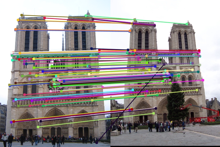
Notre Dame matched 117 out of 124 dots correctly, with 7 incorrectly for 94% accuracy.

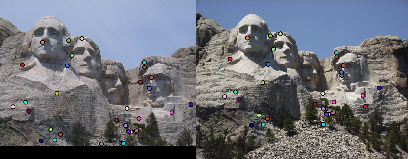
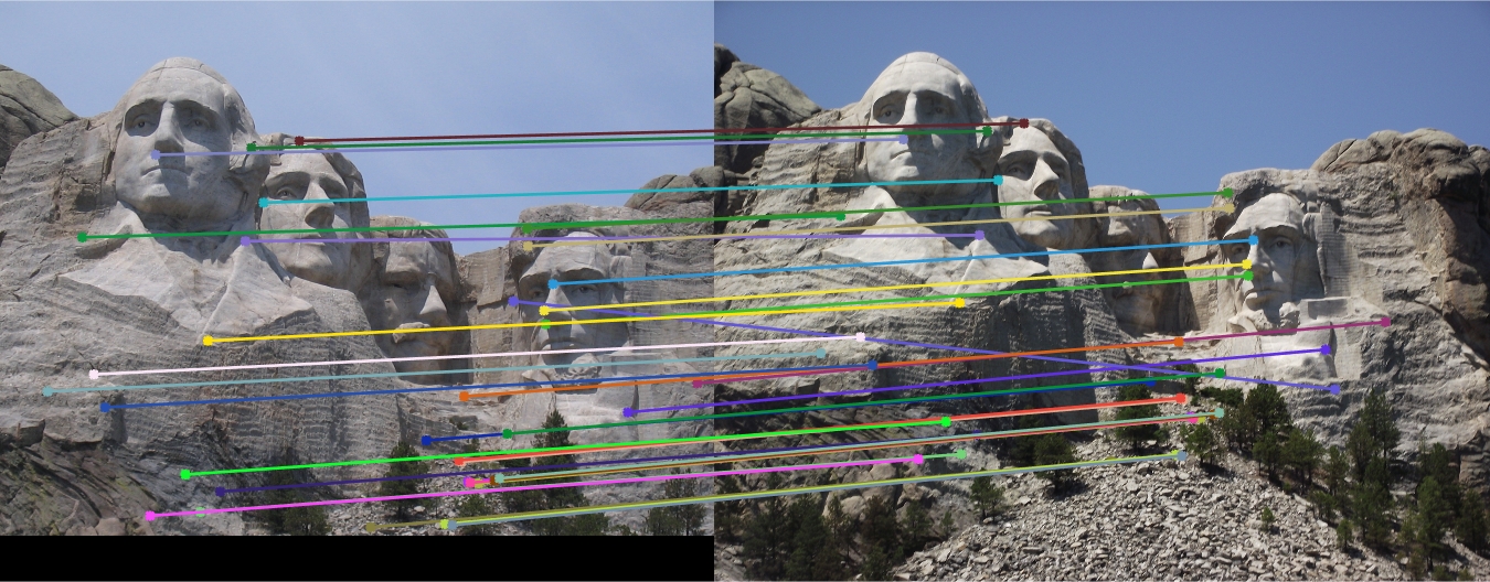
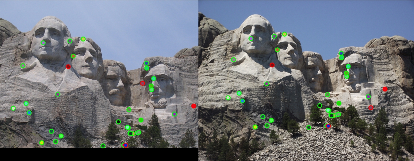
Mount Rushmore matched 31 out of 35 dots correctly, with 4 incorrectly for 89% accuracy.

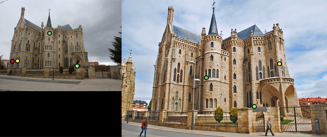
Episcopal Gaudi matched 0 out of 4 dots correctly, with 4 incorrectly for 0% accuracy.

Conclusion