Project 2: Local Feature Matching
The goal of this project is to implement feature matching in two related images. This is done in the following steps
- Interest Point Detection: Using Harris Corner Detector since corners are good interest points
- Constructing Feature Descriptor: For each interest point, we want to construct a vector representation of that point using its neighborhood
- Feature Matching: Given feature descriptors of interest points in two images, how do we match them.
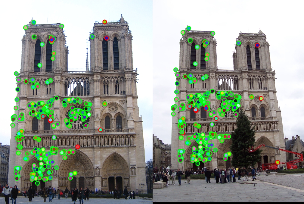
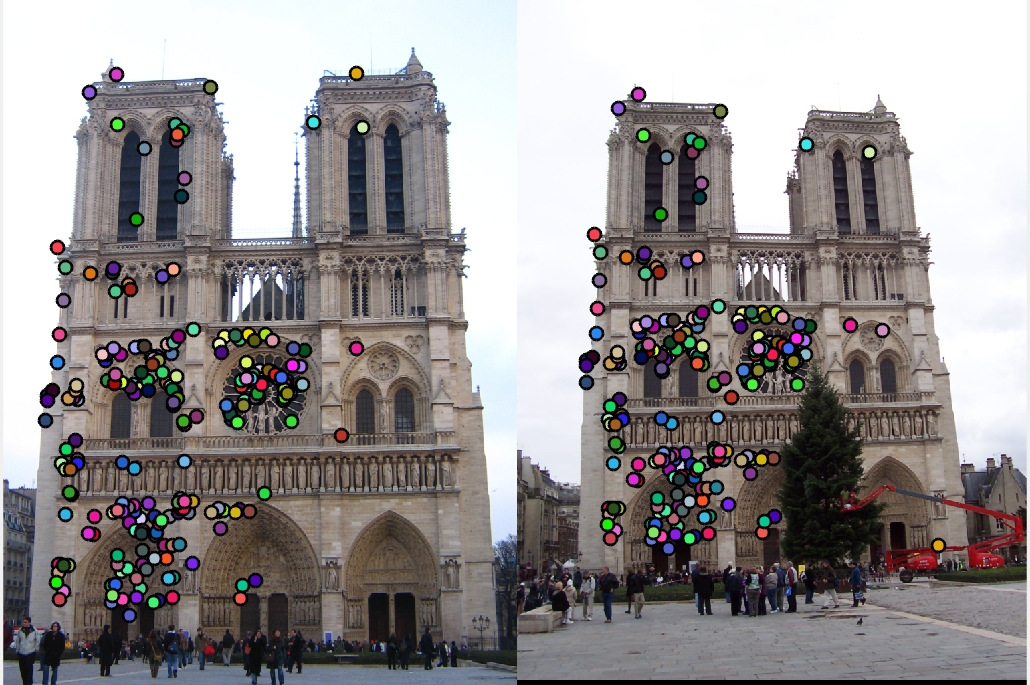
Interest Point Detection
We implement the harris corner detector
%example code
[Ix, Iy] = imgradientxy(image);
gaussian = fspecial('gaussian', feature_width, 1);

Ixx = Ix.*Ix;
Iyy = Iy.*Iy;
Ixy = Ix.*Iy;

%Convolve with a gaussian.
g_Ixx = imfilter(Ixx, gaussian);
g_Iyy = imfilter(Iyy, gaussian);
g_Ixy = imfilter(Ixy, gaussian);

alpha = 0.04;
har = (g_Ixx.*g_Iyy - g_Ixy.^2) - alpha * (g_Ixx + g_Iyy).^2;
har_max = colfilt(har, [5 5], 'sliding', @max);
har = har.*(har == har_max);
Constructing the feature descriptor
The main idea here is as follows. For each interest point we take a 16*16 frame around it. We divide it into 4*4 cells. In each cell we compute the gradient and bin the direction of the gradient in 8 possible directions. After binning we construct a histogram of gradient directions in each cell. Each cell gives a 8 dimensional vector and there are a total of 16 cells in the frame, so we get a 128 dimensional vector.
[grad_mags, grad_dirs] = imgradient(image);
grad_dirs = grad_dirs + 180; %Since gradient direction values are -180:180

%Bin the gradients
num_bins = 8;
bin_size = 360/num_bins;
grad_dirs = ceil(grad_dirs/bin_size);
grad_dirs = max(1, grad_dirs); %Handle the case when the grad is 0 degree

for index=1:num_points
  %x and y are given in coordinate system
  %xi and yi are in matrix index
  xi = y(index);
  yi = x(index);
  %Find the neighborhood around each point, the frame
  frame_x = xi - feature_width/2 + 1: xi+feature_width/2;
  frame_y = yi - feature_width/2 + 1: yi+feature_width/2;

  grad_mag_frame = grad_mags(frame_x,  frame_y); %gradient magnitudes in the frame
  grad_dir_frame = grad_dirs(frame_x,  frame_y); %gradient directions in the frame
  feature_vector = [];
  grad_mag_frame = grad_mag_frame .* gaussian;

  for i=0:3
    for j=0:3
      grad_mag_cell = grad_mag_frame(i*4+1: i*4+4, j*4+1:j*4+4); %gradient magn in the cell
      grad_dir_cell = grad_dir_frame(i*4+1: i*4+4, j*4+1:j*4+4); %gradient directions in the cell
      %This cell will create num_bin dimensional feature_vector
      cell_feature_vector = zeros(1,num_bins);

      %Flatten out the matrices.
      grad_mag_cell = reshape(grad_mag_cell, [size(grad_mag_cell,1) * size(grad_mag_cell,2), 1]);
      grad_dir_cell = reshape(grad_dir_cell, [size(grad_dir_cell,1) * size(grad_dir_cell,2), 1]);

      for u=1:size(grad_dir_cell,1);
        orientation = grad_dir_cell(u);
        cell_feature_vector(orientation) = cell_feature_vector(orientation) + grad_mag_cell(u);
      end
      feature_vector = [feature_vector cell_feature_vector];
    end
  end
end
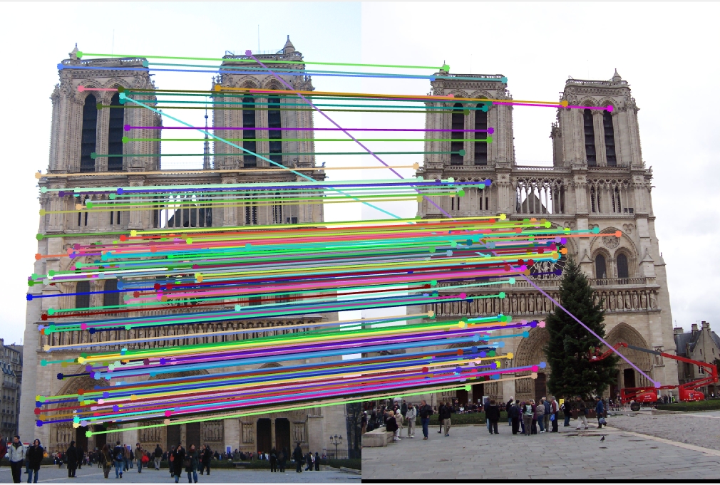
Feature matching
For feature matching we use Nearest Neighbor Distance Ratio as described in the book.Results
|
Extra Credit: PCA
We collect the images from the additional data and run PCA on the feature vectors obtained. We are basically trying to find out the most prominent dimensions of the feature vectors.
path_prefix = '../data/all_images/';
fid = fopen('../data/all_images.txt');
C = textscan(fid, '%s', 'delimiter', '\t', 'HeaderLines', 0);
fclose(fid);

feature_vectors = [];
for i=1:length(C{1})
  filename = char(C{1}(i));
  path = strcat(path_prefix, filename);
  path = char(path);
  image = imread(path);
  image = single(image)/255;
  scale_factor = 0.5;
  image = imresize(image, scale_factor, 'bilinear');
  image_bw = rgb2gray(image);
  feature_width = 16;
  [x, y] = get_interest_points(image_bw, feature_width);
  [image_features] = get_features(image_bw, x, y, feature_width);
  %Append the feature vectors
  feature_vectors = [feature_vectors; image_features];

  disp(size(feature_vectors));
  % mean normalization and scaling
  features_norm = bsxfun(@minus, feature_vectors, mean(feature_vectors));
  features_norm = bsxfun(@rdivide, feature_vectors, std(feature_vectors));

  pca_matrix = pca(features_norm); % 128 x 128 matrix
end
  pca_matrix = pca_matrix(:,1:dimensions);
  feature_vector = feature_vector * pca_matrix;