Project 2: Local Feature Matching
Algorithm
Get interest points: A Harris-Laplacian approach
In this step we pick out corner points that we can easily distinguish in the image. The first part of the algorithm follows the Harris Corner detection illustrated in the book. I use 0.04 for alpha and 0.0025 the cornerness threshold. This seems to work well as it finds a reasonable amount of points.
I also use the bwconncomp() function to return the maxixum point of a blob instead of every point in it. This makes the set of interest points more refined.
To improve the algorithm, I further use a laplacian filter to determine the scale invariance of a point returned by the Harris Corner detector. I keep only the points for which the Laplacian is extremal (larger than my "upper_sigma" or lower than my "lower_sigma"). I repeat this process for different image scales (right now the resize factors are x1, x2, x3) and group all the points I have found at different scale together. While this iterative Harris_Laplacian is slow, I'm really satisfied with its performance. I made sure that I don't count the same point twice. An interest point must be at some radius r away from any other points.
Performance: Compared to old plain Harris Corner detector, my Harris-Laplacian algorithm returns many more points (at least twice the amount) for Notre Dame. For Episcopal Gaudi, by using this approach and fiddling with different parameters, I was able to pump the accuracy from 0 %to 29% as shown in the result section below (not much but still something).
Get local feature descriptions
The implementation follows the book closely. It looks at a window frame with the interest point at the center. The window frame is divided into a 4x4 grid (16 cells). In each cell, there are 8 orientation bins. Each pixel will contribute to its corresponding bin and adjacent bins.
Performance: I kept getting a very low number of matches at first for Notre Dame. The accuracy was around 90%+ but there were less 50 than matches. I was able to fix this by experimenting with the parameters (alpha and cornerness threshold in get_interest_points, threshold for nearest neighbor distance ratio) and applying a gaussian blur filter in get_features (the filter worked amazingly in ways that I never would have expected). Interpolating the gradient measurements also helped a lot. After that, I was able to get above 100 matches easily with 85%+ accuracy.
Match features
I use the ratio test to find relatively unique feature pairs (a feature pair is considered relatively unique if those features only match closely among themselves).
Performance: I've found that 0.70 for the threshold works quite well most of the time.
And that's it!
Extra credit
- Harris-Laplacian detector for scale invariance.
- Adaptive non-maximal suppression: only detect features that are both local maxima and whose response value is significantly (delta=10%) greater than that of all of its neighbors within a radius r.
- Interpolation in feature descriptors
Results
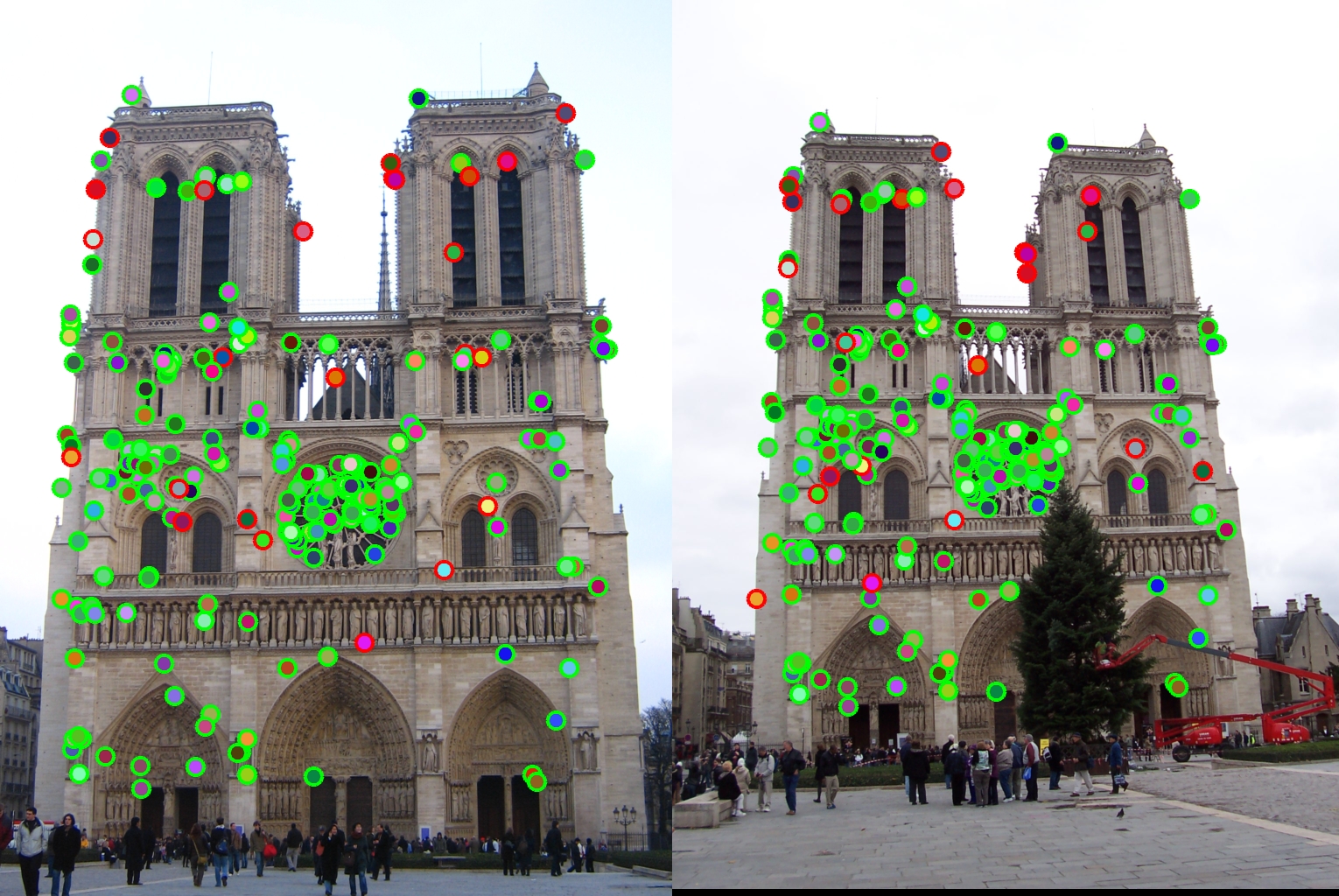
Notre Dame
195 total good matches, 24 total bad matches. 0.89% accuracy
Very good results.
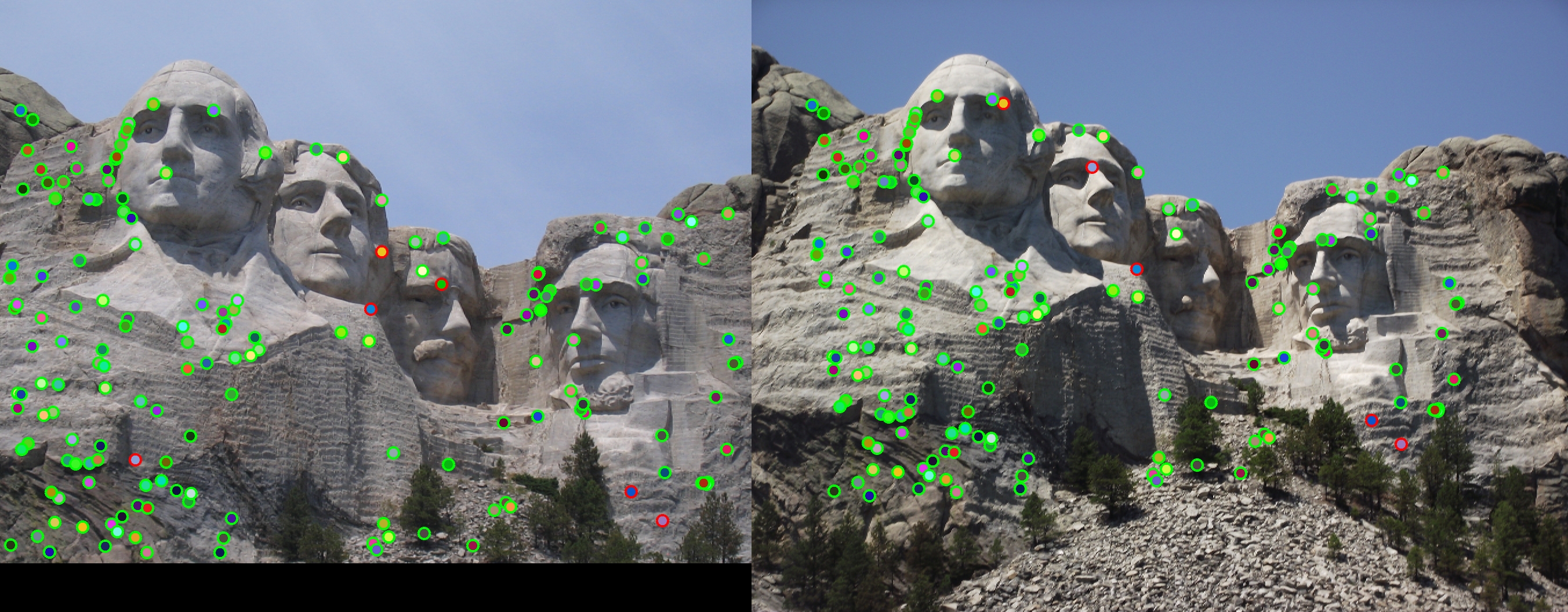
Mount Rushmore
162 total good matches, 6 total bad matches. 0.96% accuracy
The accuracy is higher on this one even though this image set appears to be hard at first glance with not a lot of sharp corners and a large difference in scale. Changing parameters can boost the number of matches over 300 while still keeping very high accuracy.
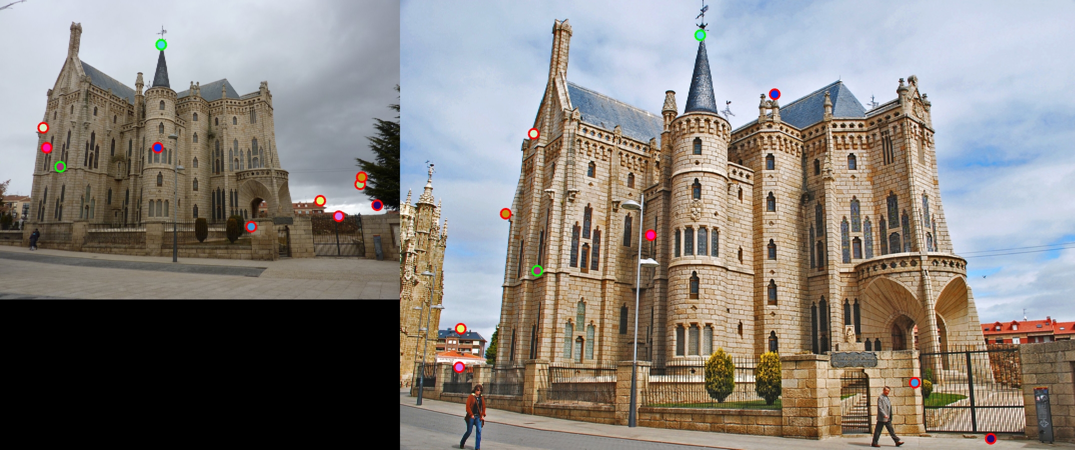
Episcopal Gaudi
4 total good matches, 10 total bad matches. 29% accuracy
Algorithm sufferred utter defeat. This image set not just has high color dissimilarity but also a big gap in scale.