Project 2: Local Feature Matching
Implementation
My basic implementation for this feature detection pipeline looks something like the following:- Harris corner detection at multiple scales.
- SIFT feature description with histogram interpolation.
- Nearest-neighbors matching and ratio testing.
Corner Detection
The corner detection is a straightforward Harris corner detector, but each point is analyzed at multiple scales in order to "guess" how big the feature is.
The scale is found by first applying a Laplacian-of-Gaussian (LoG) filter on the image, where the size of the filter corresponds to the size of features we're looking for. The LoG has the useful property of creating a high response to circles or blobs of the same size. Therefore to pick the scale of our detected points, we pick the scale with the maximum LoG response.
As a last step, we perform non-maximum suppression so that keypoints are only selected if they are the maximum in a 3x3 neighborhood.
SIFT Description
The sift descriptor works by first selecting a window around each feature that corresponds to the scale determined in the corner detection phase. The magnitudes are weighted by a Gaussian falloff with variance half the window width. This reduces the importance of gradients far away from the feature center.
The next step works by calculating the gradient around the point, then forming a 4x4x8 description of the area around the point by interpolation:
- First a histogram is made at each pixel with 8 bins from 0-360 degrees. The magnitude of the gradient is softly added to the two nearest bins whose centers are closest to the angle of the gradient. The "softly added" part means we weigh each magnitude by the distance to the bin center.
- Second, the tensor is interpolated down to 4x4 by summing the nearest neighbors to the bin, weighted by their distance from the bin center.
- Finally all vectors are projected to unit length, all values are truncated to 0.2 and then all vectors are made unit length again.
Ratio Test
To match features, we calculate the pairwise distance between each feature in two images and pick the closest pairs. In order to avoid ambiguous matches, we want to keep only the most meaningful pairs so we perform the "ratio test."
For each feature, we calculate the ratio of the closest match / the second closest match. Then we discard any matches with a ratio less than 0.7.
Results
When comparing the results with the ground truth, we can ask what was the total percentage of correct matches, but also what percentage of the top 100 matches were correct.Notre Dame
The best accuracy I achieved on Notre Dame across all matches is 92%. However, using only the top 100 matches I got as much as 95%.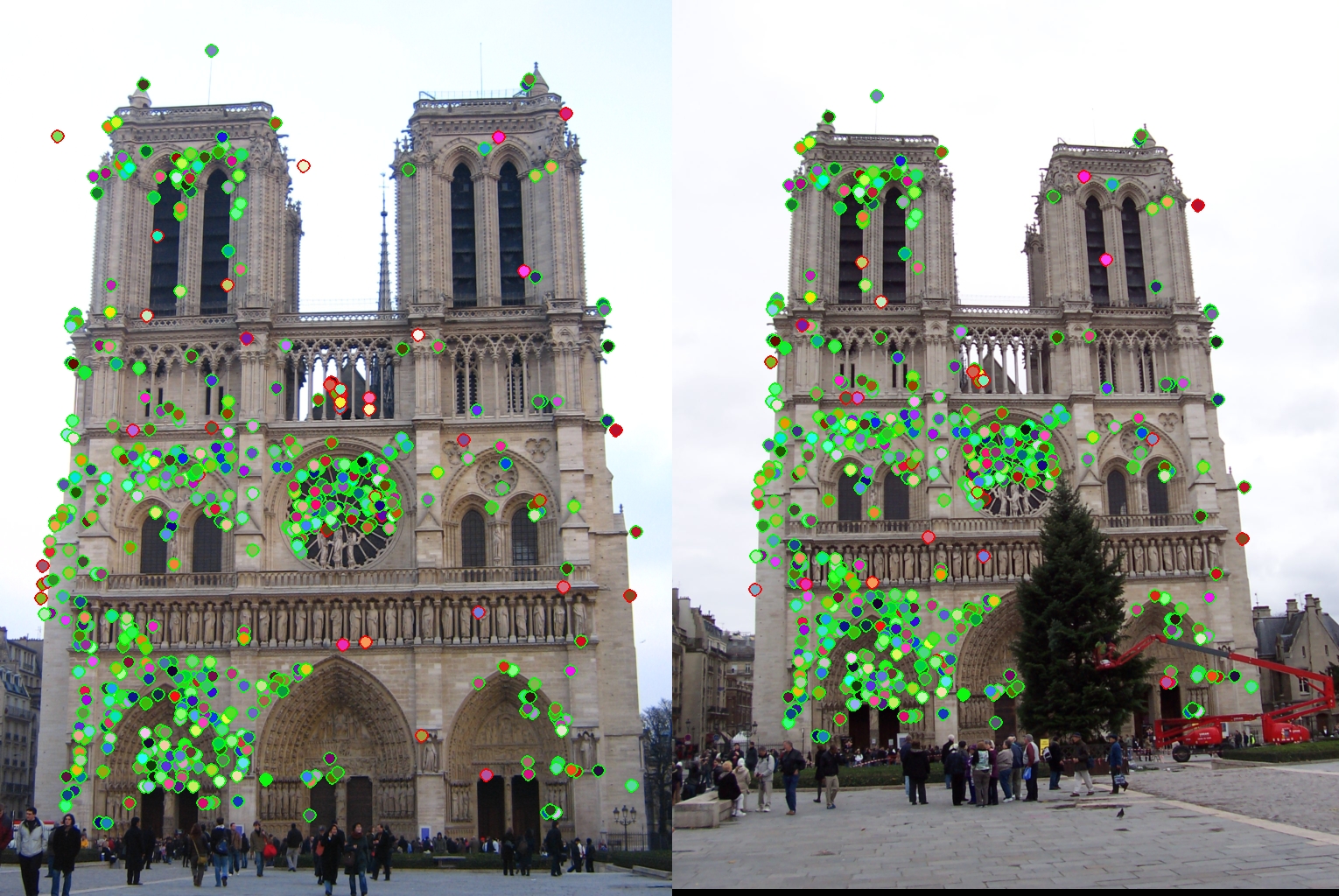
These matches were 92% accurate. The top 100 were 91% accurate.
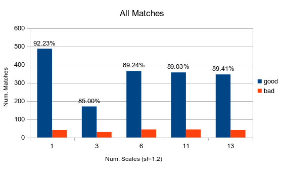
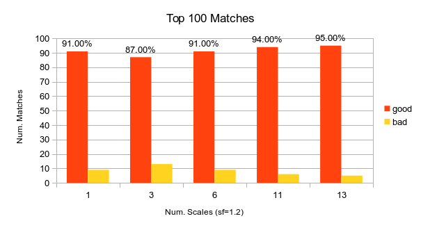
The effect of searching through scales on match accuracy.
Effect of Interpolation
One of the interesting questions I had during this project was whether or not interpolation was necessary. The original SIFT paper describes interpolation as smoothing abrupt changes in sample shifts from one histogram to another.
Using a single scale, I managed to go from 88% accuracy to 92% accuracy on all matches simply by performing the interpolation step.
Matching Gallery
Mount Rushmore
These pictures achieved extremely high accuracy without scale-invariance. Trying to make the features scale-invariant actually lowered the accuracy.
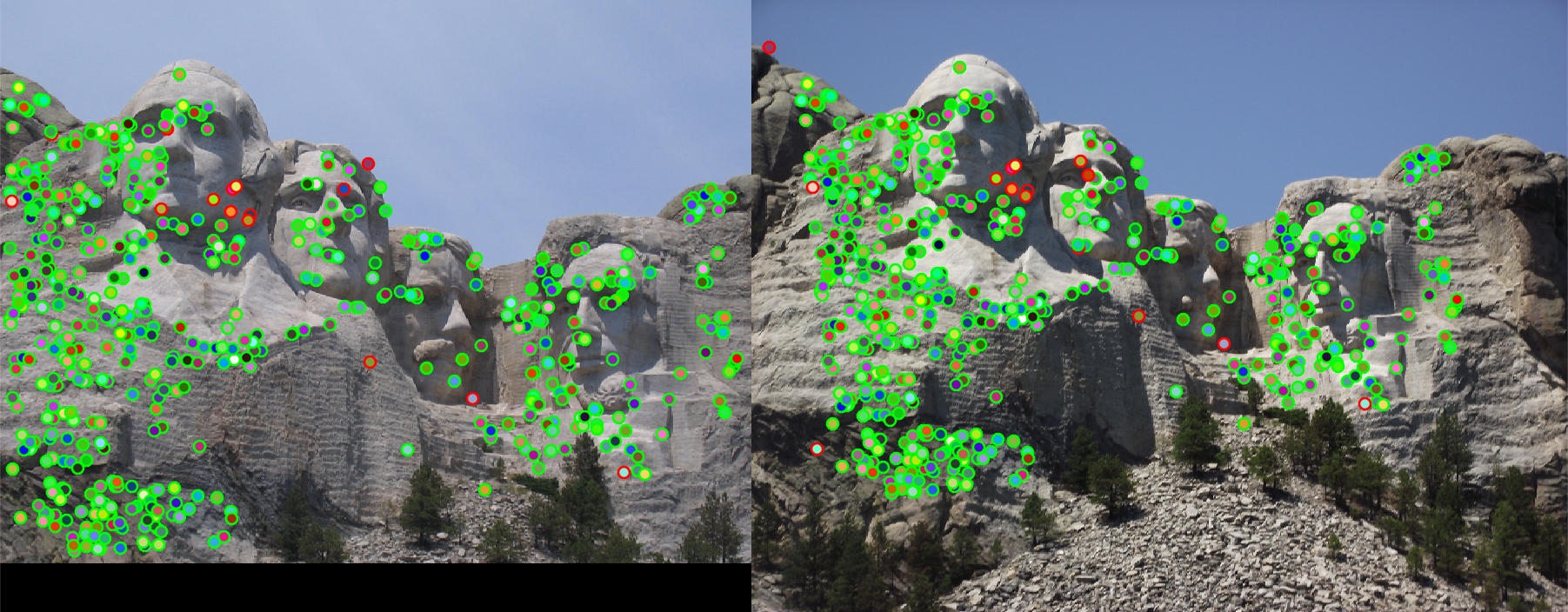
These matches were 97% accurate. The top 100 were 100% accurate. One scale is used. 511 total good matches, 15 total bad matches.
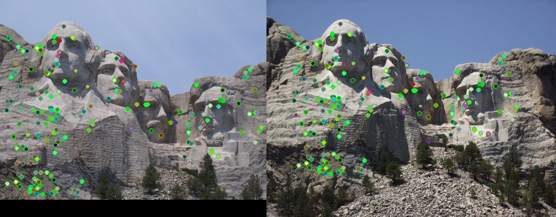
These matches were 95% accurate. The top 100 were 96% accurate. Three scales are used. 177 total good matches, 10 total bad matches.
Episcopal Palace
For these images I had to increase the ratio threshold to 0.8. Due to the pictures being at significantly different angles, my feature descriptors had a hard time making affine-invariant descriptions. Scale-invariance helped increase the accuracy.
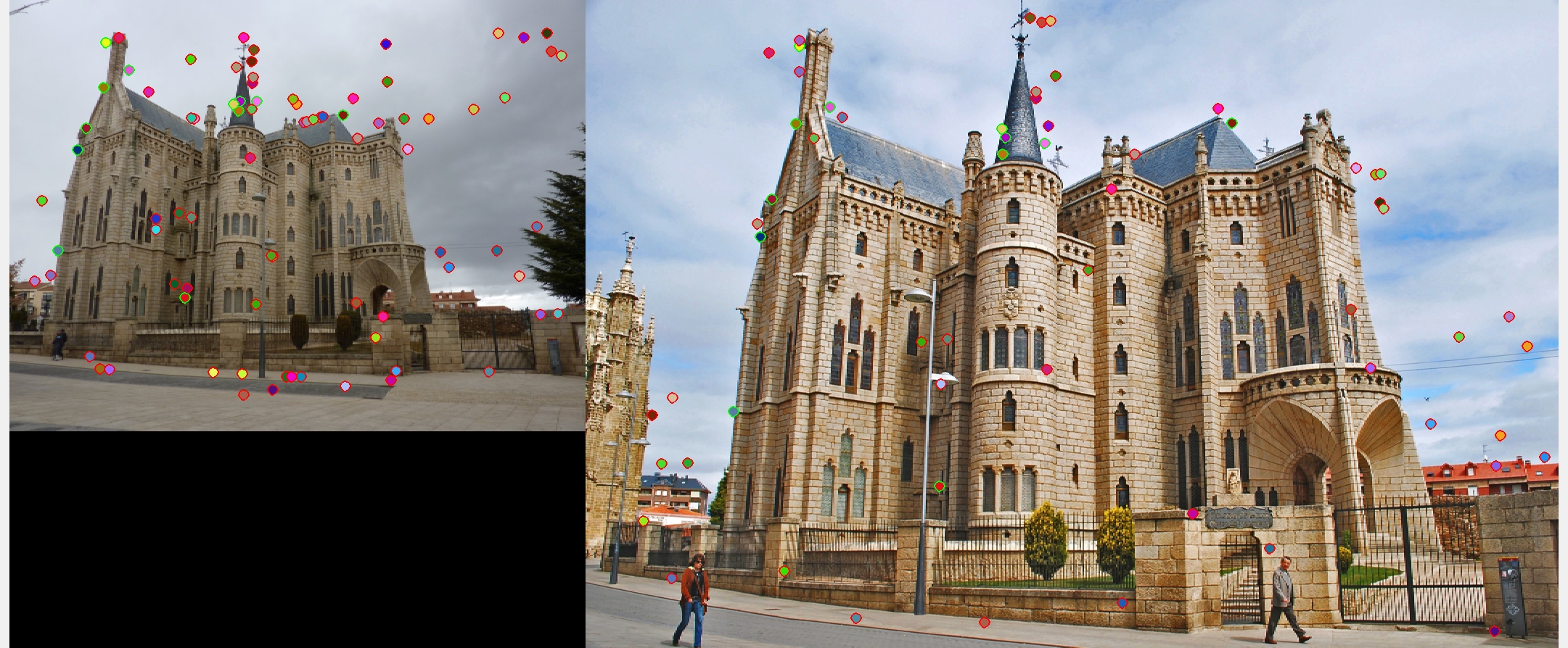
These matches were 14% accurate. One scale is used. 12 total good matches, 71 total bad matches.
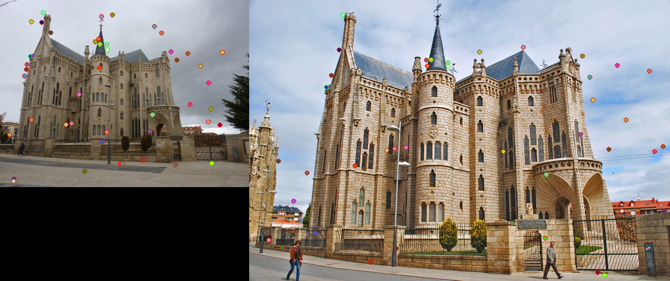
These matches were 17% accurate. Ten scales are used. 8 total good matches, 40 total bad matches.
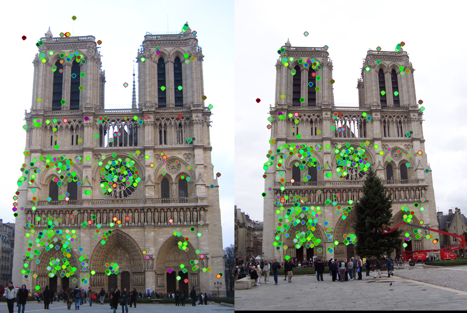
Notre Dame
These matches were 92% accurate. The top 100 were 91% accurate. One scale was used.
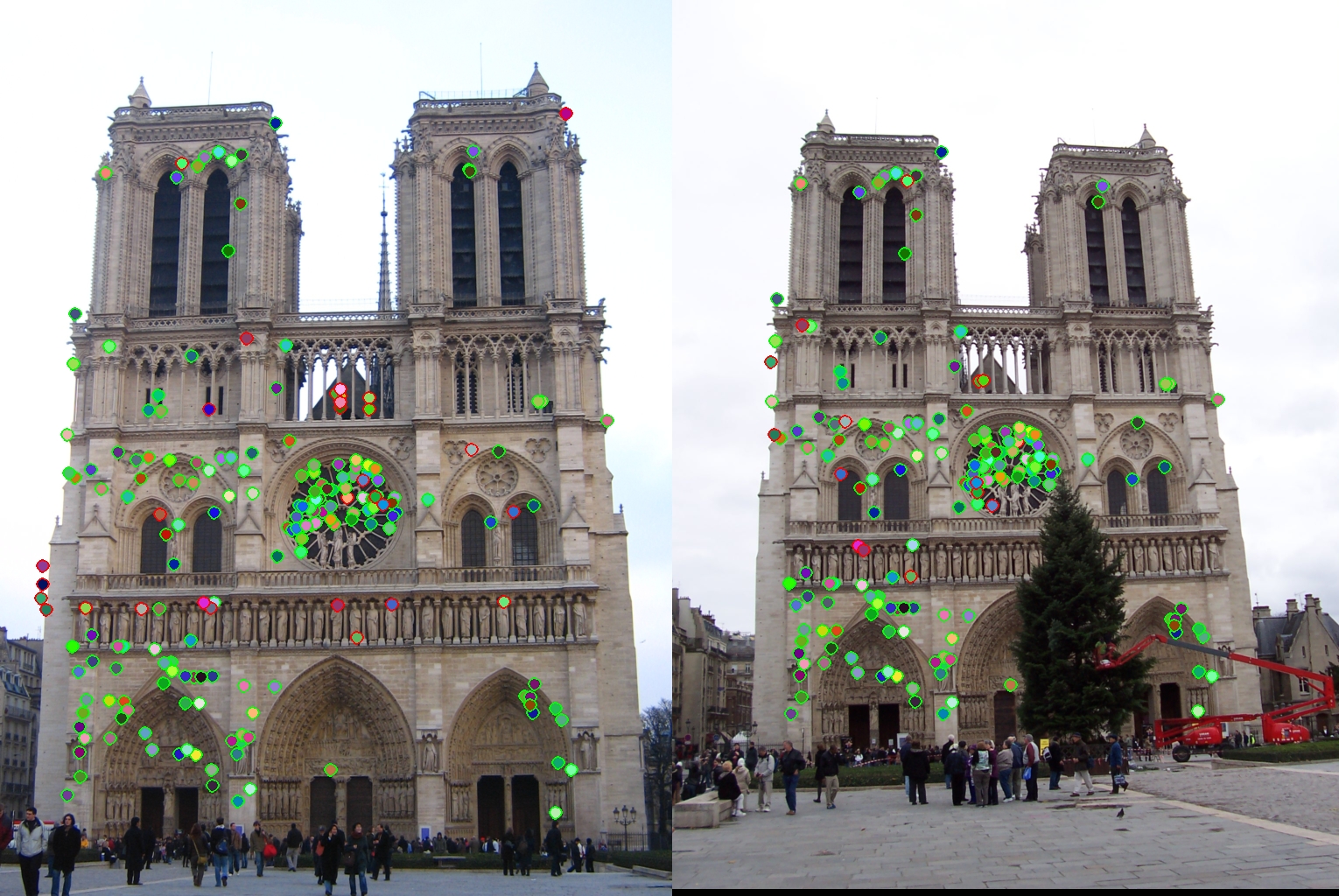
These matches were 85% accurate. The top 100 were 87% accurate. Three scales were used.
These matches were 89% accurate. The top 100 were 91% accurate. Six scales were used.

These matches were 89% accurate. The top 100 were 94% accurate. Eleven scales were used.

These matches were 89% accurate. The top 100 were 95% accurate. Thirteen scales were used.