Project 2: Local Feature Matching
Project 2 is all about matching two images of the same landmark based on similar features that exist in both images. This is challenging because the images can be taken from different angles, the landmarks may have different surroundings, the weather and thus the lighting of the photo may be different, etc. Luckily we have learned some steps in class in order to make a pipeline that helps get around these differences.
Interest Point Detection
Detecting interest points is the first step of matching images. We want to try to detect specifically corners, or places where the image gradient changes in direction dramatically, so that it is easier to match that same location to the other image later. This is done in this project using Harris corners, a technique that uses the blurred derivative of an image and the eigenvalues there of to find interest points. We then have to threshold any points we find by a particular value, in order to make sure we don't have too many and that the ones we have are the best matches. We also take the maximum of an area of pixels (in the case of my project I used a 5x5 block) to represent the actual interest point.
Local Feature Description
The second step of the pipeline is determining a way to describe an interest point that was found in step one. We need a measure that we can use to compare interest points across the image to determine if we have a match. In this project, we use a simplified version of the SIFT pipeline. This is a technique that takes a feature (in this project given by a 16x16 block around the interest point) and then separates it into a 4x4 grid of cells (in this case each cell is a 4x4 grid of pixels). We then compute a histogram with 8 bins relating to 8 orientations of the gradient of that cell (which correspond to ranges of angles of the gradient). We end up with 8 bins per cell, with 4*4=16 cells, so 16*8 = 128 parts of our feature.
Feature Matching
The last step is to actually match the features we have found and computed values for. This is done by finding which two features from the second image are closest to each feature in the first image. Closest means computing the Euclidean distance, though that does not mean how close the actual pixels are, but more so how close the feature descriptions are to one another. We then compute the ratio of these "nearest neighbor" distances. A small ratio means that the closest feature was the only feature that was remotely close to the feature in image one, and also a more likely match. By sorting all of the ratios that we compute for all the features in image one, we can get a good idea of which features are most likely to match, and discard ones that are not as likely.
Results
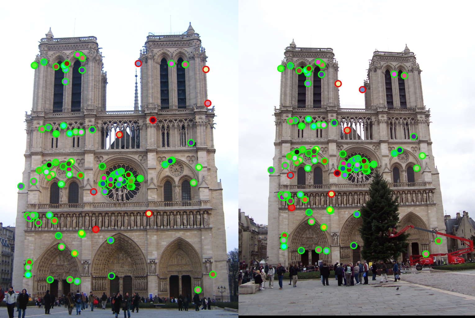
The provided images of Notre Dame matched using my project implementation, with an accuracy of 92%.
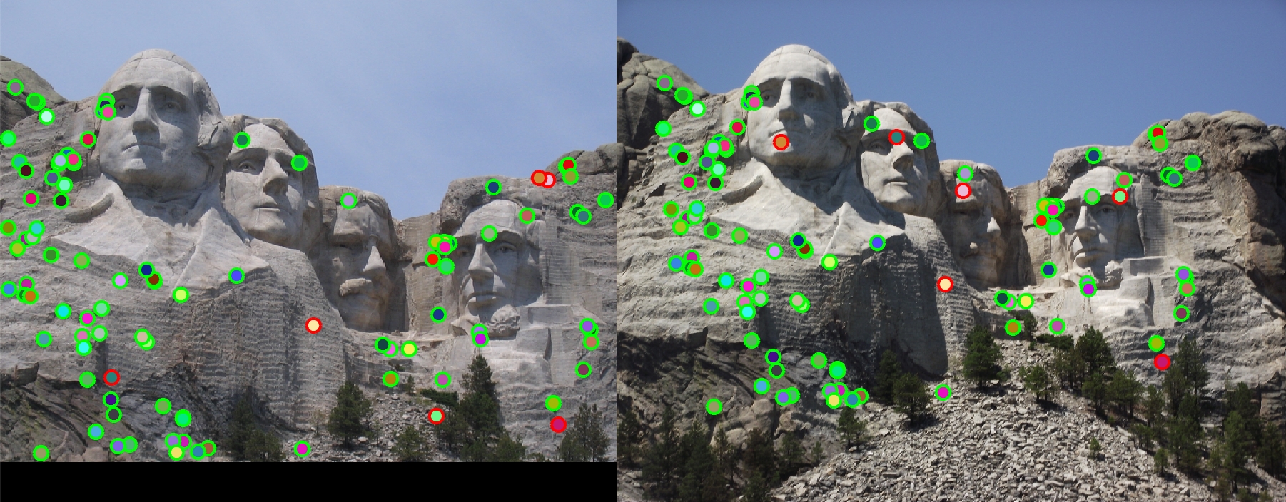
The provided images of Mount Rushmore matched using my project implementation, with an accuracy of 94%.
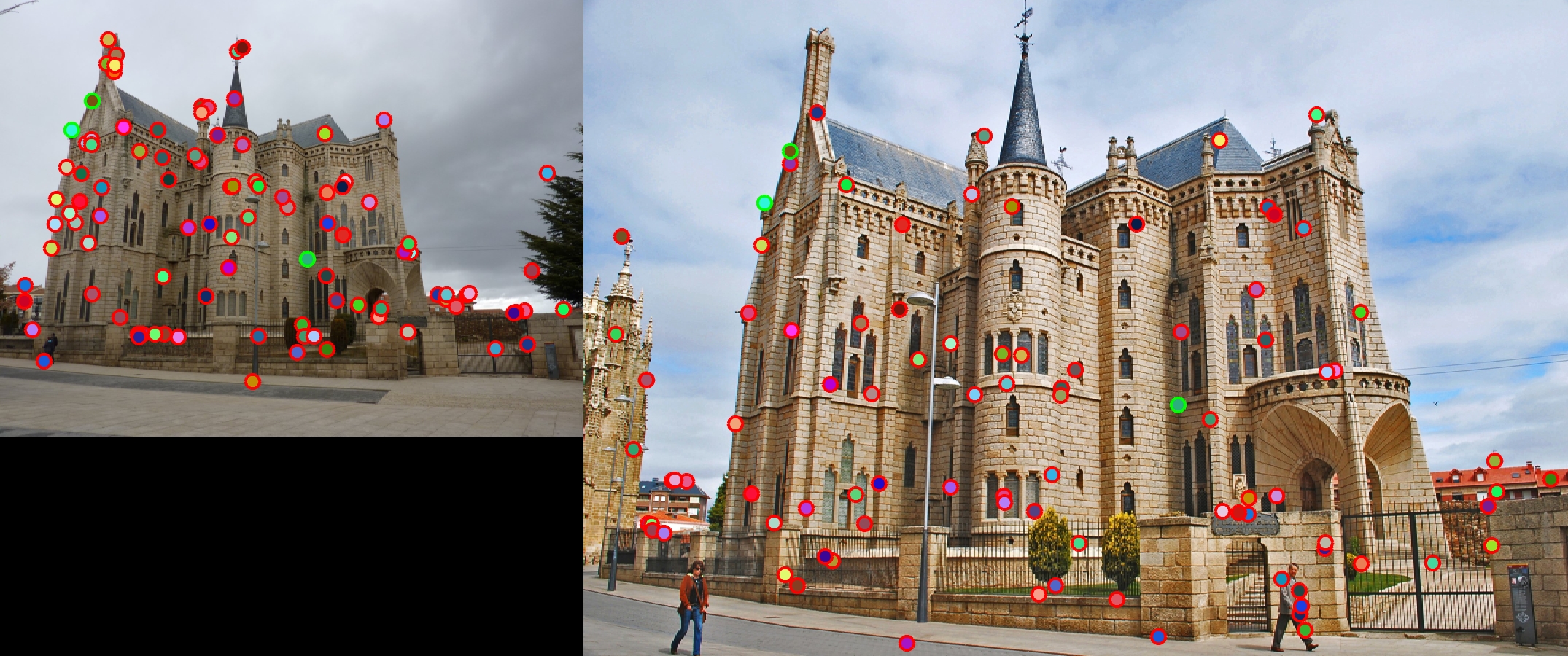
The provided images of Episcopal Gaudi matched using my project implementation, with an accuracy of 3%.
The first two sets of images I was able to achieve extremely high accuracy rates, 92% for Notre Dame and 94% for Mount Rushmore. This makes sense as the pieces of the building are different enough that calculating gradients in 8 orientations as our feature description is a good enough descriptor. You can see that most of the incorrect matches are to areas on the building that look similar, even though they are in different areas. Unfortunately, I am only getting 3% accuracy on the third set of images, representing Episcopal Gaudi. My theory is that because this landmark has lots of repeating patterns, the descriptor we used isn't specific enough and thereby matches incorrectly a large portion of the time. You can also see another building off to the left in the second image of Episcopal Gaudi that also skews the point matching, as this building does not appear in image one.