Project 2: Local Feature Matching
Getting the Interest Points
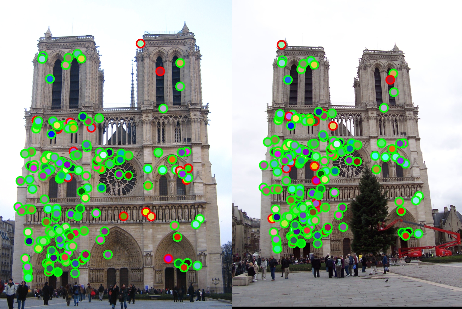
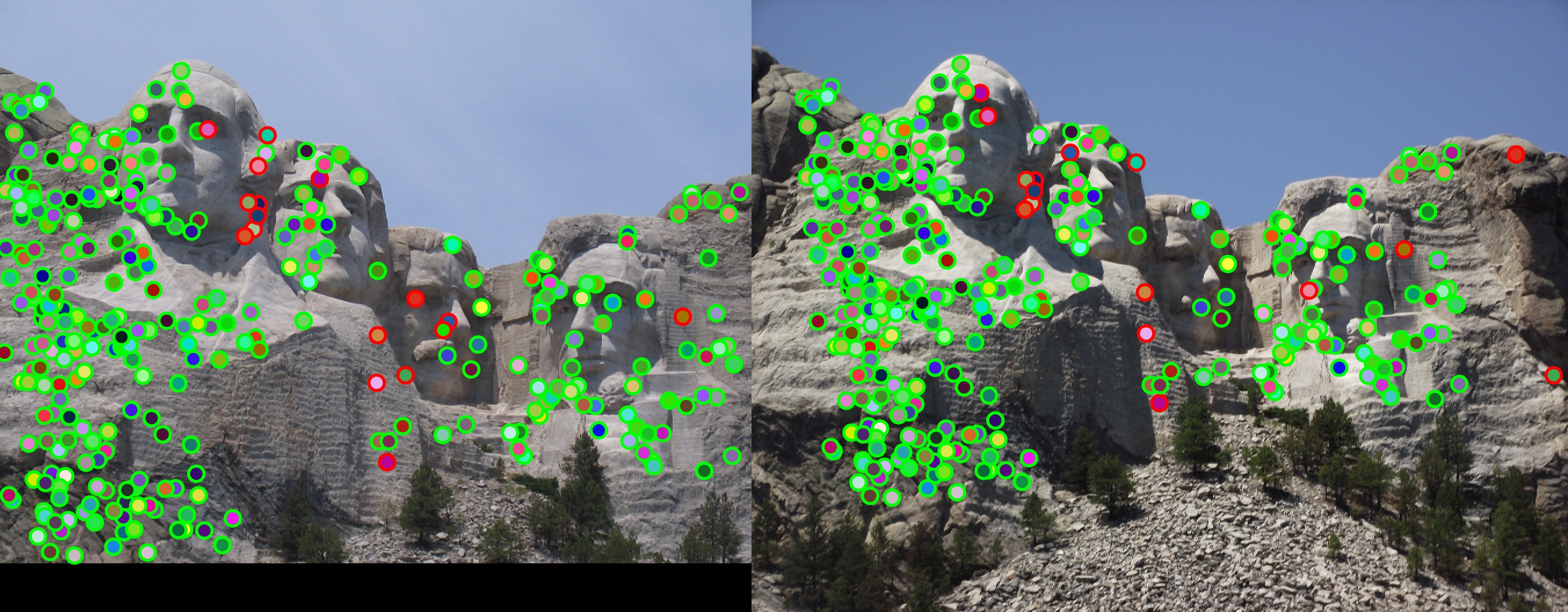
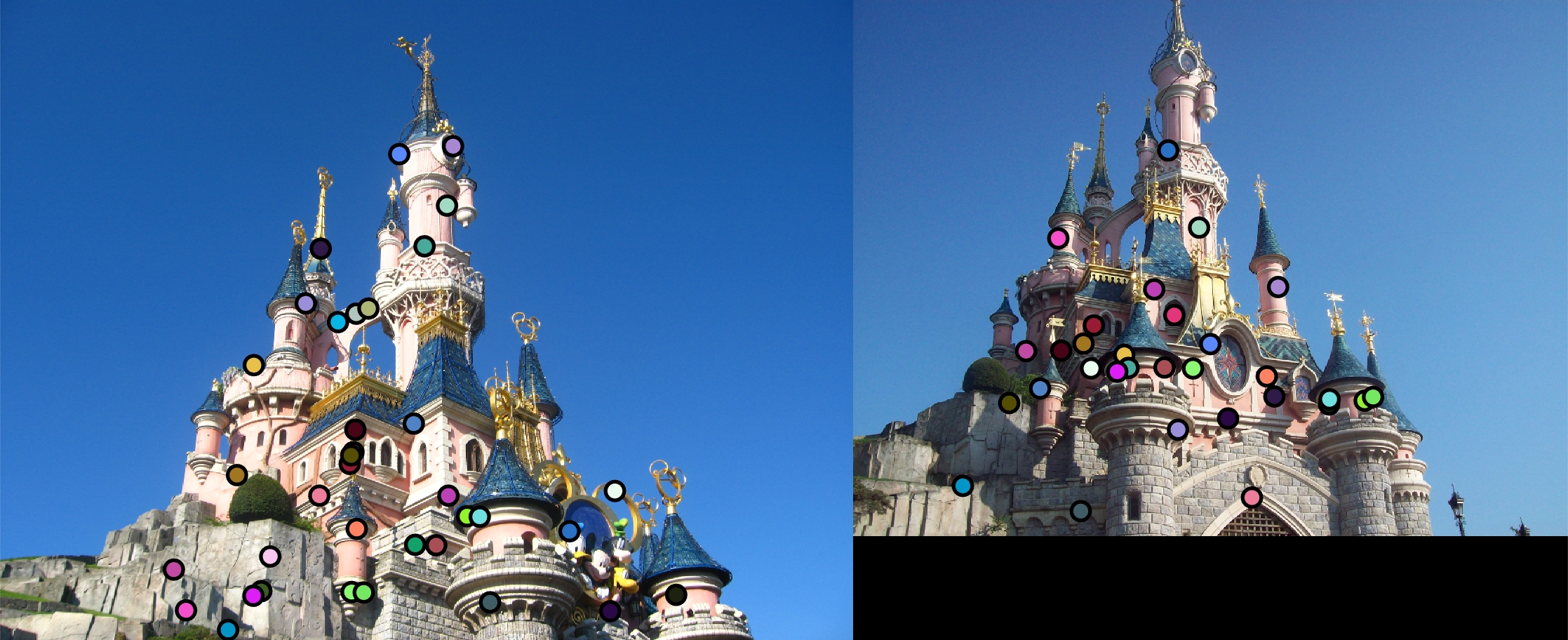
To get interest points for each image, the Harris Corner Detection algorithm is used. The gradient for each image is first calculated. The cornerness score is calculated for each pixel in the image using the equation g(I^2 x)g(I^2 y) - [g(I x * I y)]^2 - 0.06[g(I^2 x) + g(I^2 y)]^2. Next, I calculate the maximum cornerness value in a 12 x 12 neighborhood for each pixel. I chose 12 x 12 after playing with the values, as a larger neighborhood will end up yielding a lower number of more accurate interest points. After that, I iterate through the pixels of the image to get the cornerness score at each pixel. If that score is larger than the threshold of 0 (chosen after testing different values, including a dynamic threshold equivalent to the mean value of all cornerness scores) and the score is equal to the maximum cornerness value in the pixel neighborhood, add that pixel as a point of interest.
xSize = size(image, 1);
ySize = size(image, 2);

I_x2 = gradX.^2;
I_y2 = gradY.^2;
I_xy = gradX.*gradY;

g_x2 = imgaussfilt(I_x2);
g_y2 = imgaussfilt(I_y2);
g_xy = imgaussfilt(I_xy);

h = g_x2 .* g_y2 - g_xy.^2 - 0.06 * (g_x2 + g_y2).^2;

thresh = 0;
maxIm = colfilt(h, [12,12], 'sliding', @max);

for xI=1:xSize
   for yI=1:ySize
       hVal = h(xI, yI);

        if (hVal > thresh && hVal == maxIm(xI, yI))
            x = cat(1, x, yI);
            y = cat(1, y, xI);
            confidence = cat(1, confidence, hVal);
        end
   end
end
Getting the Features
To get the feature for each interest point, first the gradient of the image is calculated. From there, a feature_width x feature_width grid of pixels is pulled, with the interest point centered in the grid. If part of the grid is outside of the image, the interest point is simply discarded to prevent incorrect features. From there, the feature_width x feature_width grid is then divided into a 4 x 4 grid of cells. The gradient at each pixel is then put into a 8-bin histogram based on the direction of the gradient. No position interpolation is performed. Each magnitude is simply added to the overall bin value. For each histogram, the values are then normalized. After that, the histogram for each pixel in the cell is appended, creating a (feature_width / 4)^2 * 8 size feature.
[gradX, gradY] = imgradientxy(image);
[gradMag, gradDir] = imgradient(gradX, gradY);

points = size(x, 1);

half_width = feature_width / 2;

features = zeros(points, (feature_width / 4)^2 * 8);

for i=1:points
    % To ensure there is a ceil and a floor
   xVal = y(i);
   yVal = x(i);

   % Determining range for pixels in feature_width x feature_width
   % neighborhood
   xValCeil = ceil(xVal);
   xValFloor = floor(xVal);
   yValCeil = ceil(yVal);
   yValFloor = floor(yVal);

   if (xValCeil == xValFloor)
       xValCeil = xValCeil + 1;
   end

   if (yValCeil == yValFloor)
       yValCeil = yValCeil + 1;
   end

   xMin = xValFloor - (half_width - 1);
   xMax = xValCeil + (half_width - 1);
   yMin = yValFloor - (half_width - 1);
   yMax = yValCeil + (half_width - 1);

   if (xMin > 0 && yMin > 0 && xMax <= height && yMax <= width)
       % Getting the feature_width x feature_width gradient neighborhood
       gradMagNeighborhood = gradMag(xMin:xMax, yMin:yMax);
       gradDirNeighborhood = gradDir(xMin:xMax, yMin:yMax);

       % Iterating through the 4x4 grid
       gridWidth = feature_width / 4;

       feature = [];

       for j=1:4
           for k=1:4
              hist = zeros(1, 8);

              startLocX = 1 + (j-1) * gridWidth;
              startLocY = 1 + (k-1) * gridWidth;

              gridMag = gradMagNeighborhood(startLocX:startLocX+gridWidth-1, startLocY:startLocY+gridWidth-1);
              gridDir = gradDirNeighborhood(startLocX:startLocX+gridWidth-1, startLocY:startLocY+gridWidth-1);

              gridMag = imgaussfilt(gridMag);

              for l=1:gridWidth
                  for m=1:gridWidth
                      binNum = floor(((mod(gridDir(l,m) + 180, 360)) / (360 / 8))) + 1;
                      hist(1, binNum) = hist(1, binNum) + gridMag(l,m);
                  end
              end

              hist = hist/norm(hist);
              feature = cat(2, feature, hist);
           end
       end

       features(i,:) = feature(1,:);
   end
end
Matching the Points
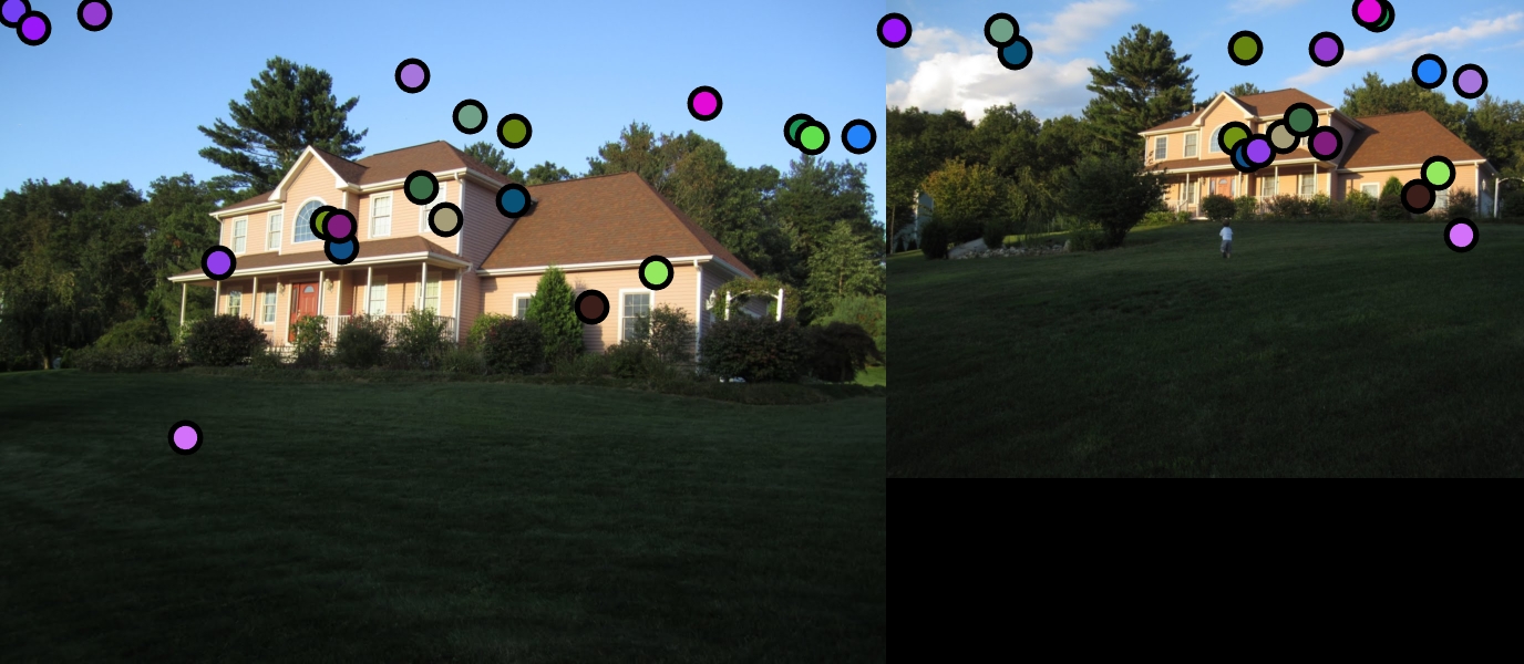
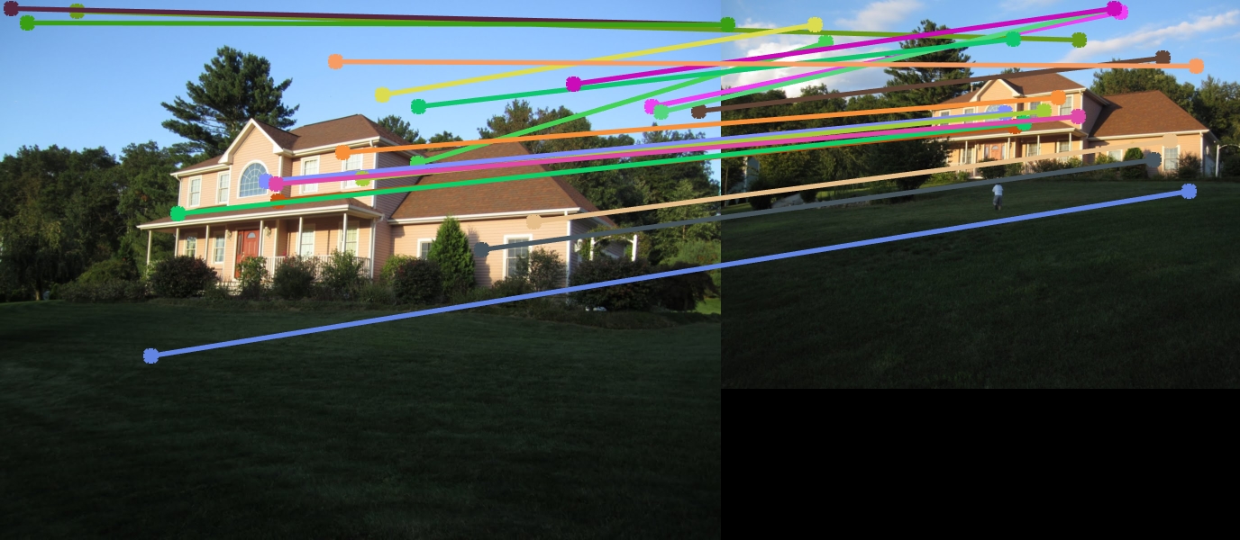
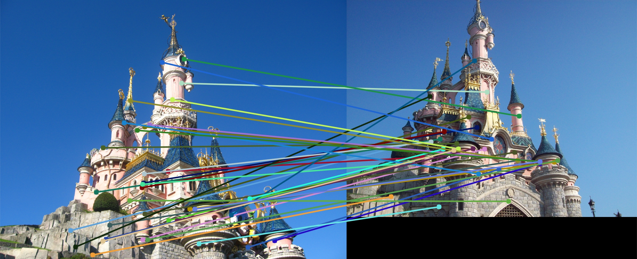
To match features between the two images, a Euclidean distance is calculated for each possible pair of features. Then for each feature in the first image, the feature that has the smallest distance in the second image is selected as the corresponding point. Then, a ratio is calculated to determine confidence of the match. The ratio takes the smallest distance pair for the feature and divides it by the second smallest distance pair. The smaller the ratio, the more confident the match is. After this, the features are filtered to only allow matches with a confidence better that 80%, throwing out unconfident matches.
matches = [];
confidences = [];

for i=1:num_features1
    d1_feature1 = -1;
    d1_feature2 = -1;

    d1 = realmax;
    d2 = realmax;

    for j=1:num_features2
        diffs = features1(i,:) - features2(j,:);
        diffSq = diffs .* diffs;
        dist = sqrt(sum(diffSq));

        if (dist < d1)
            % Shifting d1 to d2
            d2 = d1;

            d1 = dist;
            d1_feature1 = i;
            d1_feature2 = j;
        else
            if (dist < d2)
                d2 = dist;
            end
        end
    end

    if (d1_feature1 > 0 && d1_feature2 > 0 && d1 / d2 < 0.8)
        matches = cat(1, matches, [d1_feature1, d1_feature2]);
        confidences = cat(1, confidences, d1 / d2);
    end
end