Project 2: Local Feature Matching
This project covers local feature detector and matching for images. Specifically, the Harris corner detection algorithm is used to identify points of interest, a Scale-Invariant Feature Transform (SIFT)-like feature is used to describe features of the image independent of scaling and orientation, and a Nearest Neighbor Distance Ratio algorithm is used to match features in two images of the same thing.
Interest Point Detection
The first part of this assignment was to implement the Harris Corner Detector algorithm. This algorithm works as follows:
- Identify areas of high contrast in the X and Y direction of the image by finding the image derivatives in each direction. In my case, I did this by applying a convolution filter to the image: [-1 0 1; -1 0 1; -1 0 1]. This filter was used for the X direction (Fig. 1), and its transpose was used in the Y direction (Fig. 2). I also tried using a Sobel filter, but found that my filter was more effective.
- Trim edge values for each image derivative to avoid spurious interest points.
- Square the X and Y derivative matrices, and find the X * Y matrix. Create an auto-correlation matrix, [ XX XY; XY, YY ], using these values (Figs 1-3).
- Blur the image derivatives with a Gaussian filter. I had the best results using a 3 by 3 kernel, and sigma = 1.
- Apply the Harris corner response function to the auto-correlation matrix for eigenvalue analysis. This function returns high values where the "cornerness" is strong in an image.
- (I used a sliding block filter to find the maximum values returned by the Harris equation, and returned the X and Y values corresponding to those locations.)
% Find value for Harris Detector Matrix
det_M = (Ix_squared .* Iy_squared) - (Ix_Iy .* Ix_Iy);
harris = det_M - 0.04 * (Ix_squared+Iy_squared).*(Ix_squared+Iy_squared);

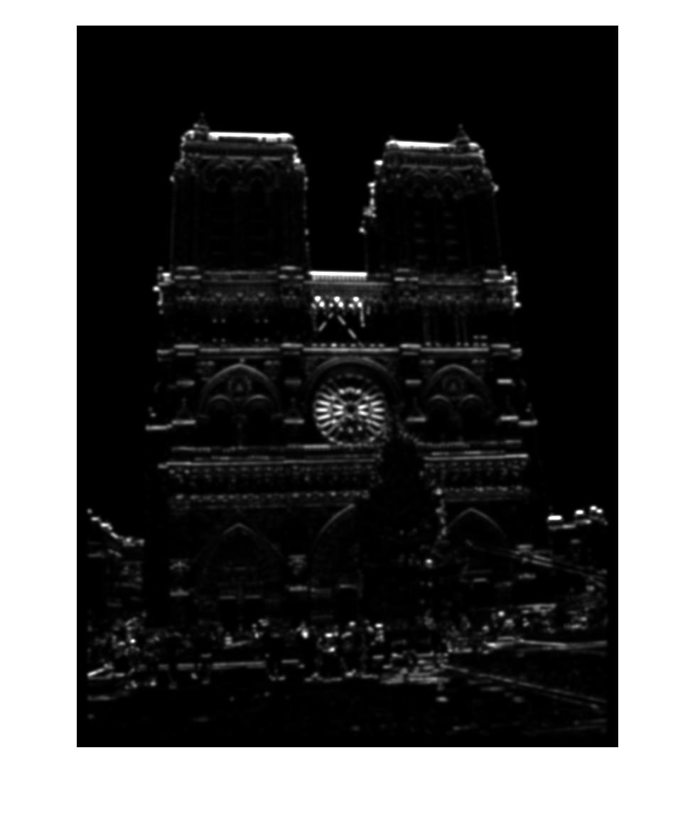
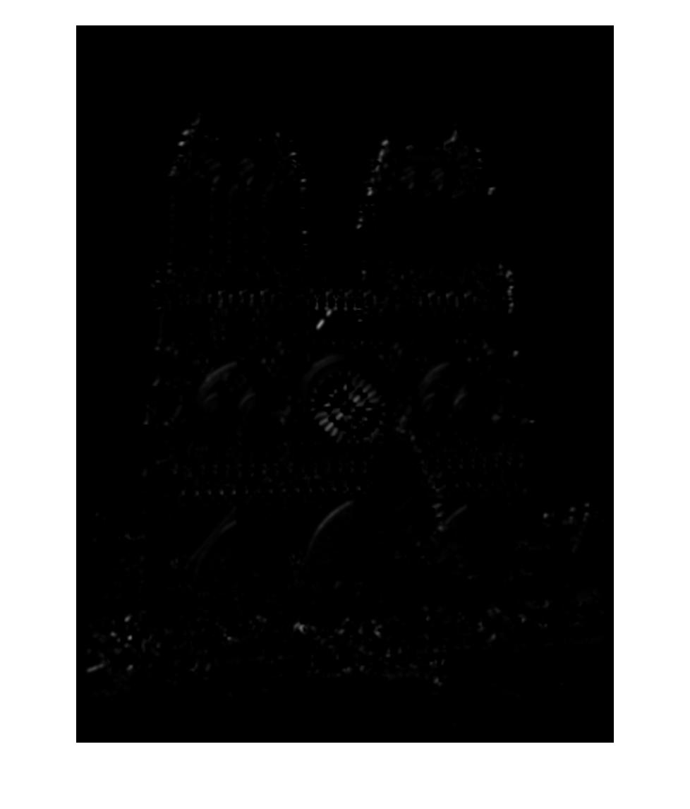
Fig. 1 (left): image derivative in the X direction, squared. Fig. 2 (center): image derivative in the y direction, squared. Fig. 3 (right): X derivative multiplied by Y derivative. All images blurred with Gaussian filter.
This function returns a list of "interest points" corresponding to potentially identifying locations in the image. It also returns a list of confidences based on the value returned by the Harris corner response function for each respective location.
Local Feature Description
Once a set of interest points has been extracted from an image, those interest points must be represented, or described, in a way that allows them to be compared to points in other images. A Scale-Invariant Feature Transform (SIFT)-like feature allows the points to be represented as histograms of oriented gradients weighted by magnitude. I first found the directional gradients for the image, then the magnitudes of the directional gradients, as well as an orientation matrix for the image. For each interest point, a window of length and width feature_width is constructed, analyzed in blocks of size 4 x 4, and for each block, the gradient histogram is computed, multiplied by the locational magnitude, and saved to a features matrix.
Feature Matching
The Nearest Neighbor Distance Ratio test was used to determine which features of two images corresponded to the same location. This involves finding the distance to the closest "neighbor", or matching feature, as well as the distance to the second closest neighbor, and finding the ratio of these two distances. A small ratio indicates that the feature is a good match. I used a threshold of 0.7 for testing, with the idea being that only matches with ratios below this value would be returned. Smaller values resulted in too few matches being returned, and larger values led to a decrease in accuracy (which can be mitigated by returning only the top 100 or so results).
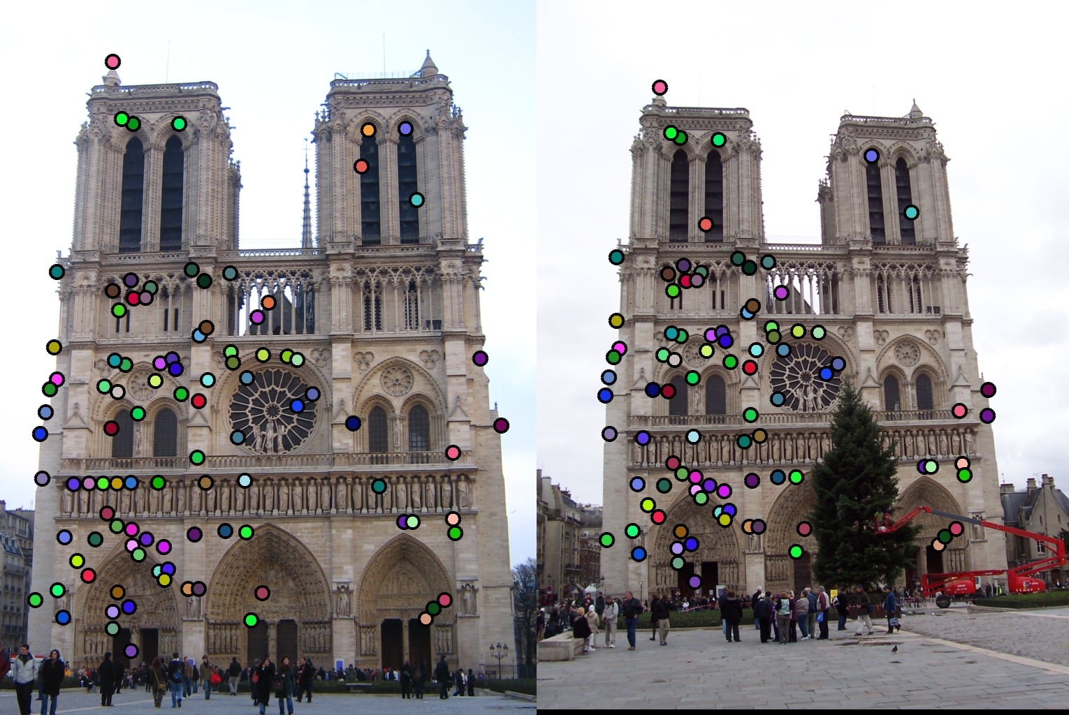
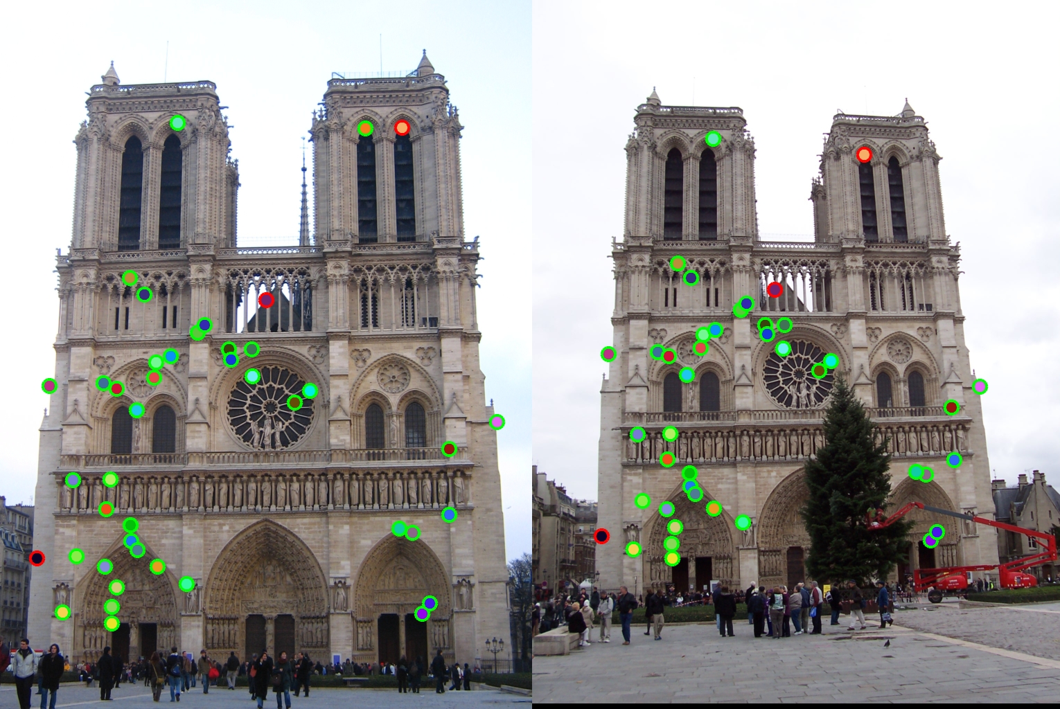
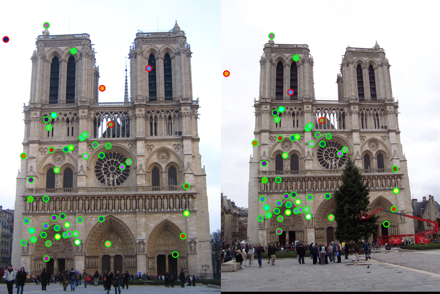
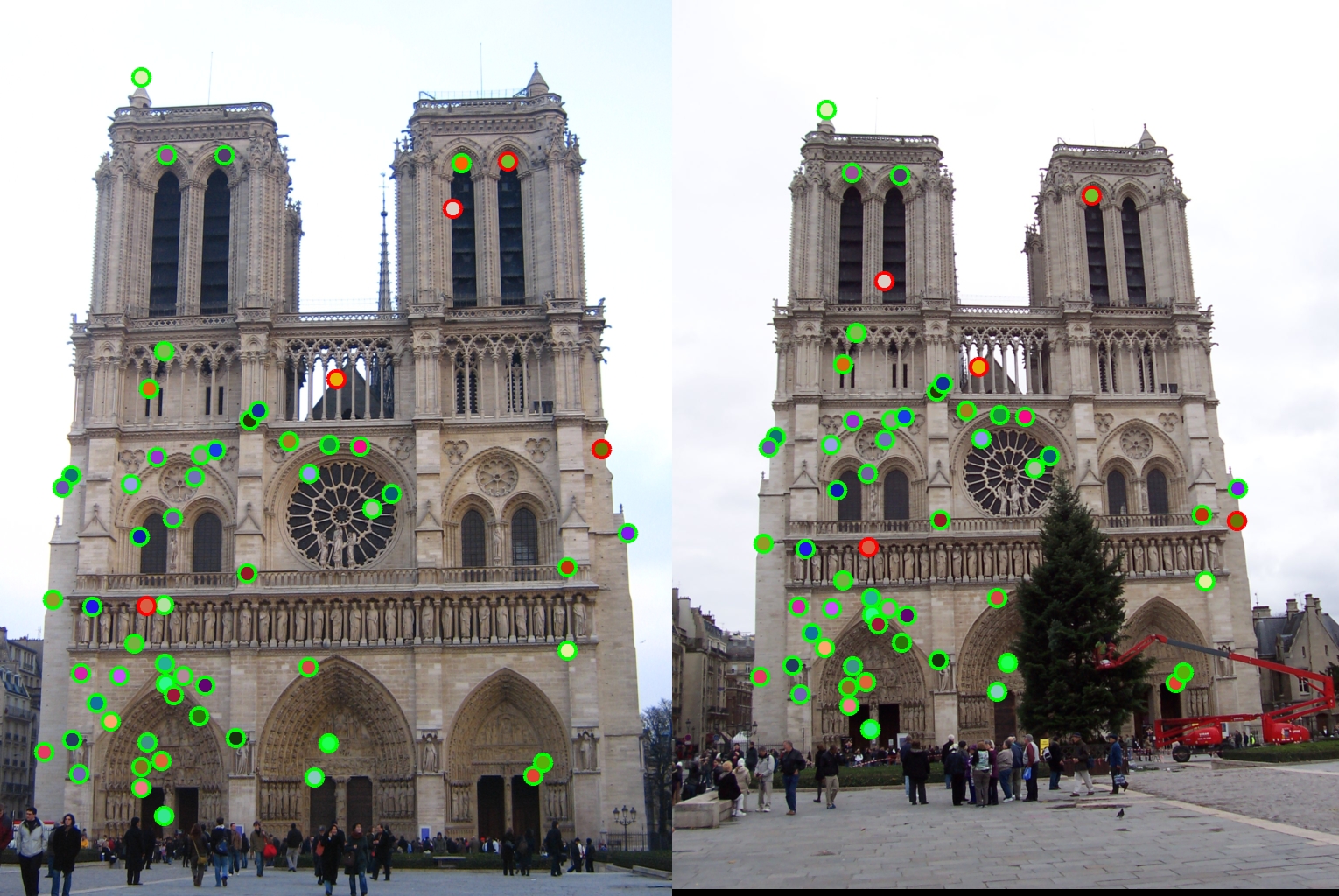
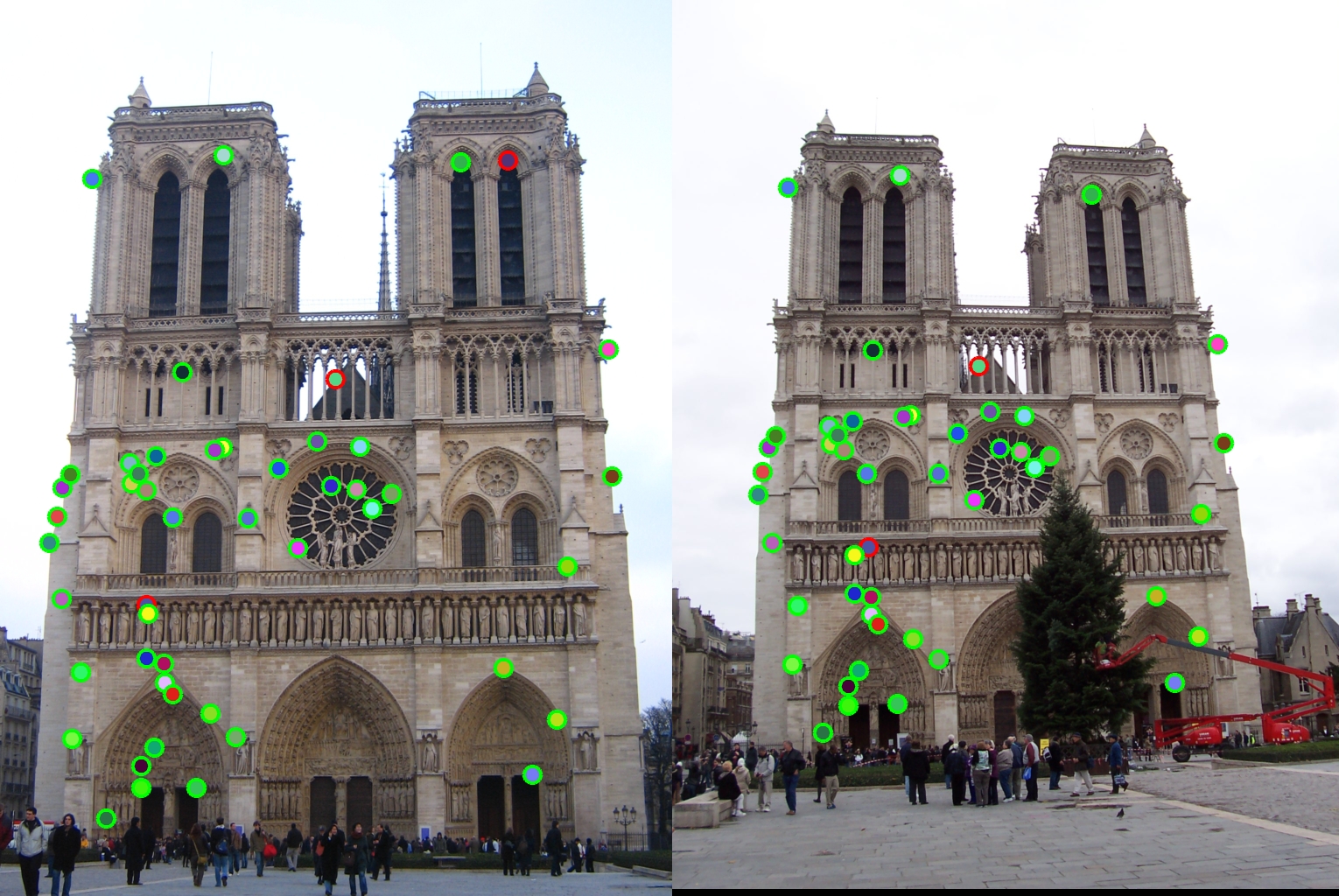
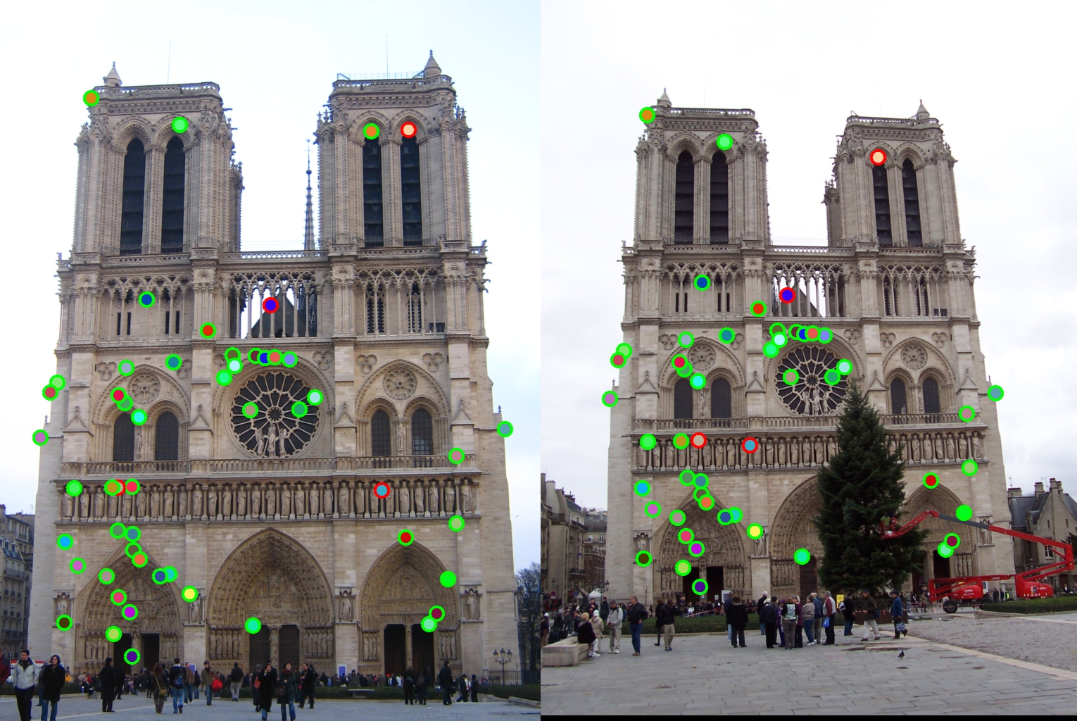
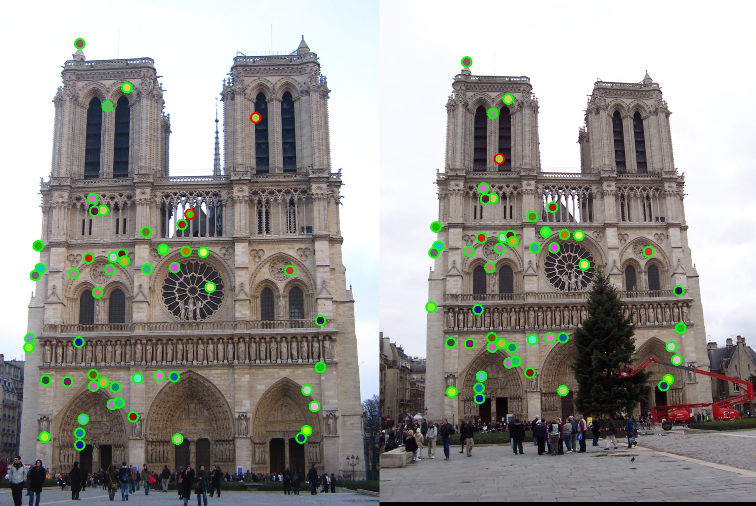
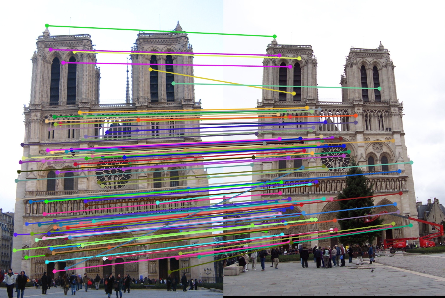
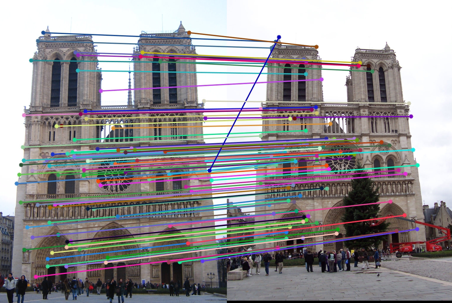
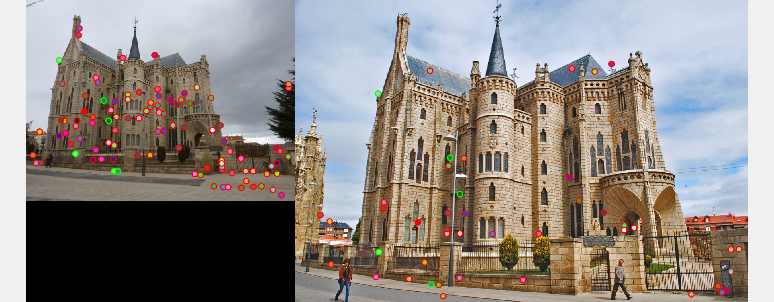
Fig. 4. Notre Dame images with their matches circled.
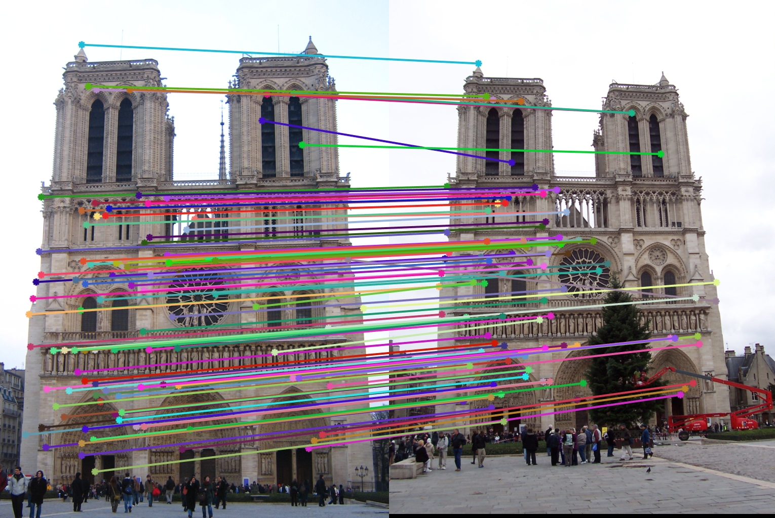
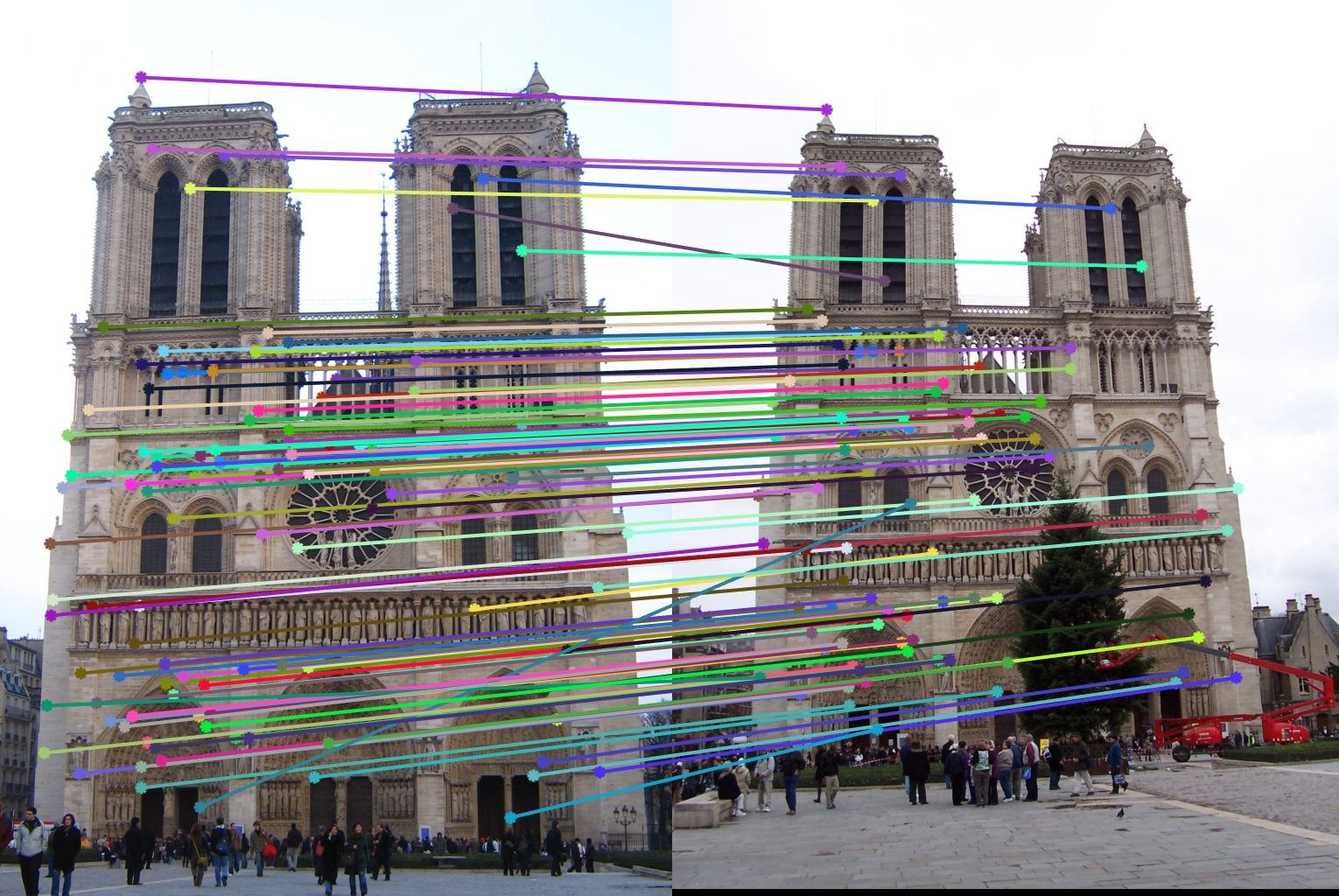
Fig. 5. Notre Dame images with arrows indicating matches.
Results and Optimizations
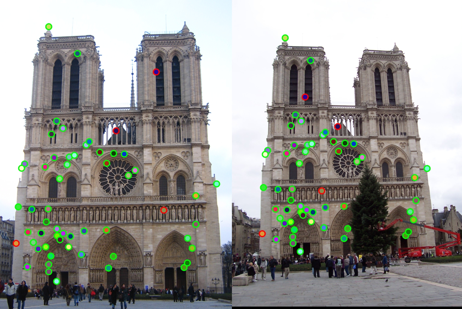
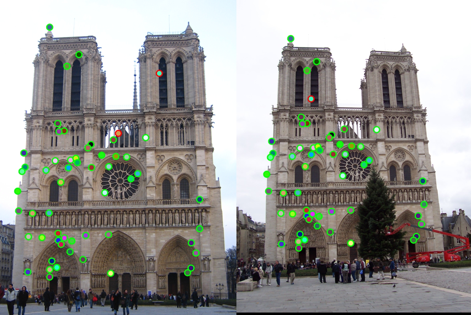
Fig. 6. Notre Dame matching with default parameters. 53 matches returned, 93% accuracy.
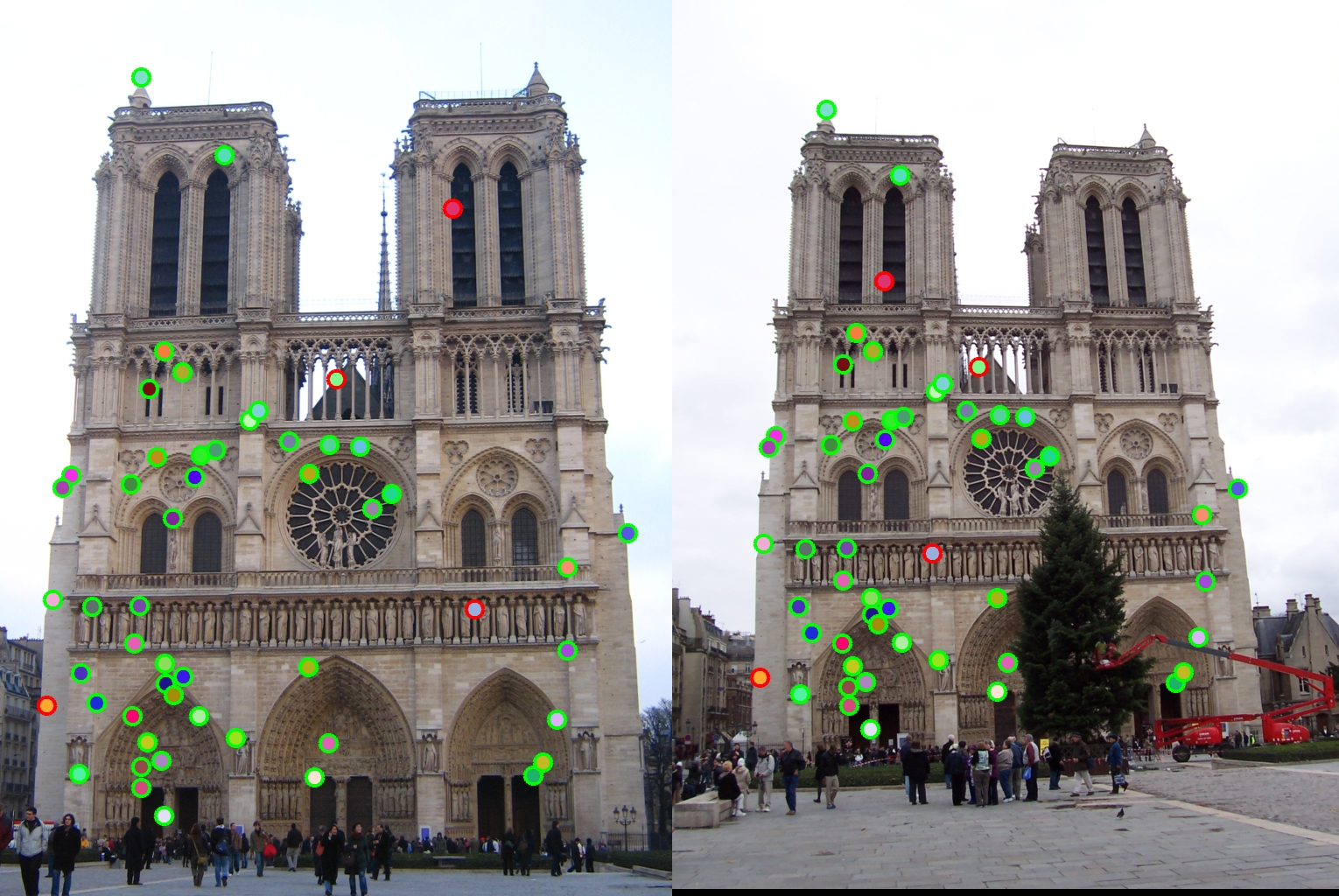
I was able to achieve different results by manipulating the values for alpha, Gaussian blur parameters, the Harris filtering value, and the factor I raised the features to in get_features. The results for each of these are discussed below, using the Notre Dame image as an example. While each variable is being manipulated, the value for alpha is fixed at 0.04, Gaussian blur fixed at [3, 3] with sigma = 1, feature factor fixed at 0.6, and Harris filtering value fixed at 0.5. There is a threshold of 0.7 set so that different number of results can be seen.
Alpha
|
Gaussian Blur
|
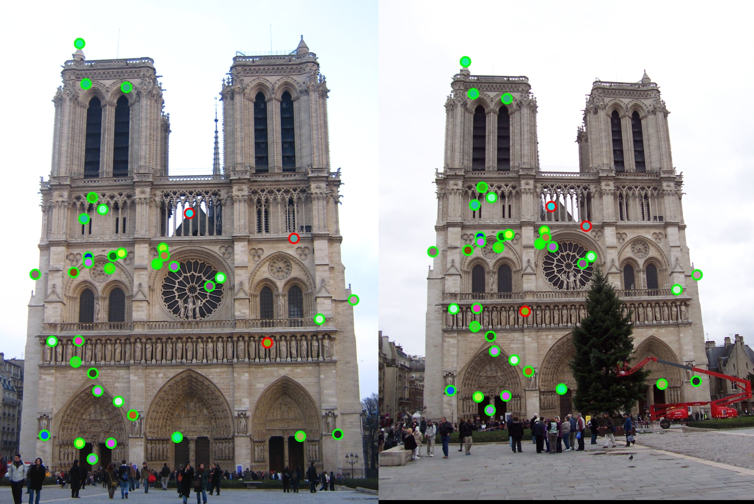
Fig. 8. Left: Size = 3 by 3, sigma = 2: 60 matches returned, accuracy = 92%. Center: Size = 6 by 6, sigma = 1: 49 matches returned, accuracy = 94%*. Right: Size = 15 by 15, sigma = 1, 53 matches returned, accuracy = 92%.
Harris Filtering Value
% Assign threshold for standout values
threshold = harris > 0.5 * mean2(harris);
harris = harris .* threshold;

|
Fig. 9. Left: Value = 1: 53 matches returned, accuracy = 92%. Center: Value = 5: 38 matches returned, accuracy = 92%. Right: Value = 10: 34 matches returned, accuracy = 94%.
Features Raised to a Factor
features = features .^ 0.6;
|
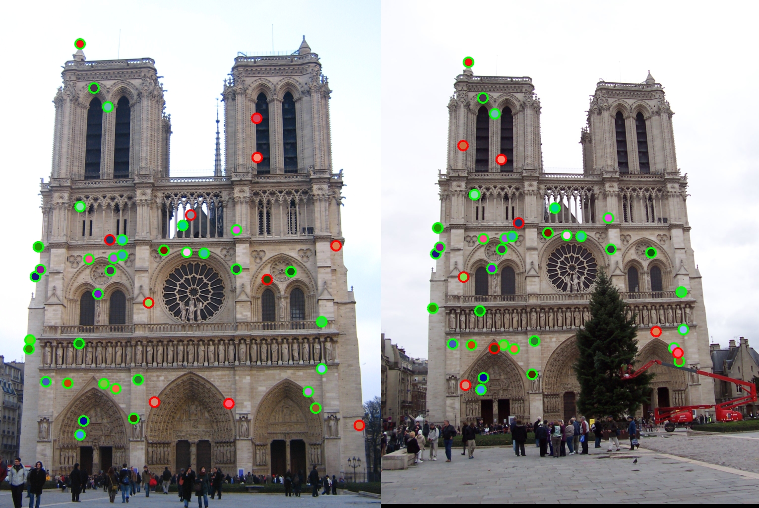
Fig. 10. Left: Not raised to a factor: 53 matches returned, accuracy = 96%*. Center: Value = 0.8: 57 matches returned, accuracy = 96%*. Right: Value = 1.5: 45 matches returned, accuracy = 78%.
After running these tests, there were a few values that returned better results than my default values. Specifically, a kernel size of 6 by 6 performed better than the size of 3 by 3, and raising the features matrix to the power 0.8 was more accurate and returned more results than my default value of 0.6. To test this theory, I ran the code with my default and the new values for the Mount Rushmore images, and ran it with no threshold set (returning the top 100 points).
Mount Rushmore
|
Top 100 Matches
|
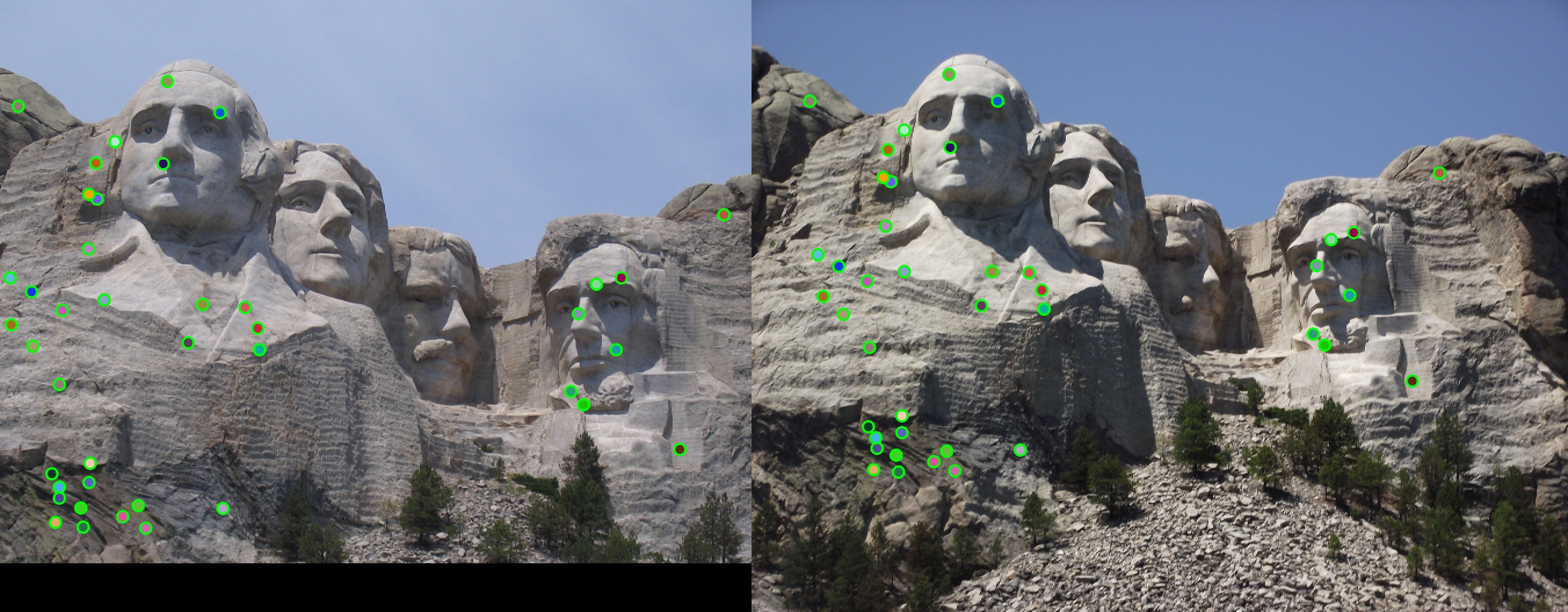
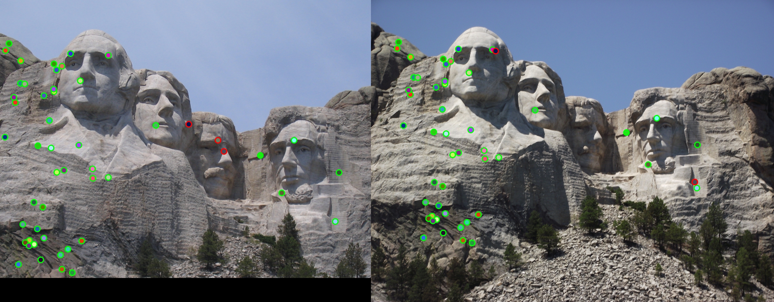
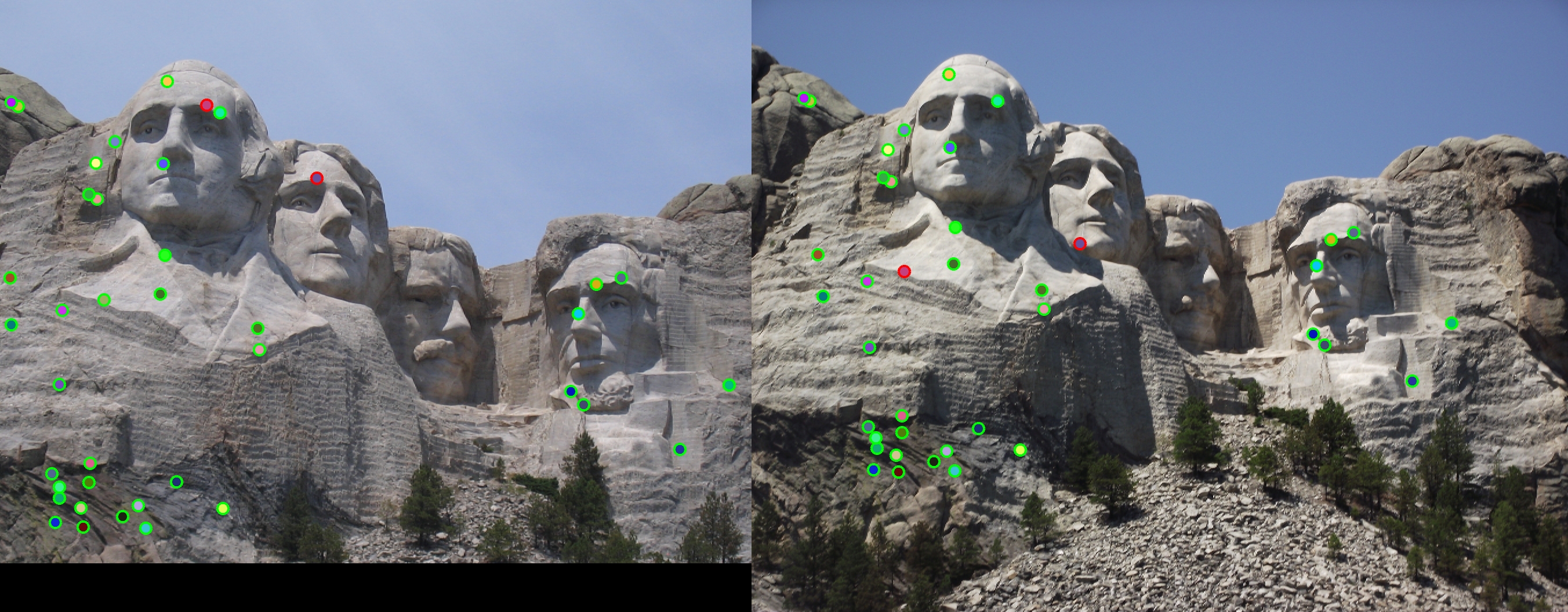
Fig. 12. Left: default values, 100 matches returned, accuracy 94%. Center: size = 6 by 6, 100 matches returned, accuracy = 89%. Right: features matrix raised to 0.8: 100 matches returned, accuracy = 90%.
The above results show that my default values perform best overall given different images or scenarios. Using these parameters, I have run my code on different image sets.
Episcopal Gaudi
|
Fig. 13. My code did not work as well on this image. It only achieved 6% accuracy, likely due to the variation in shading.
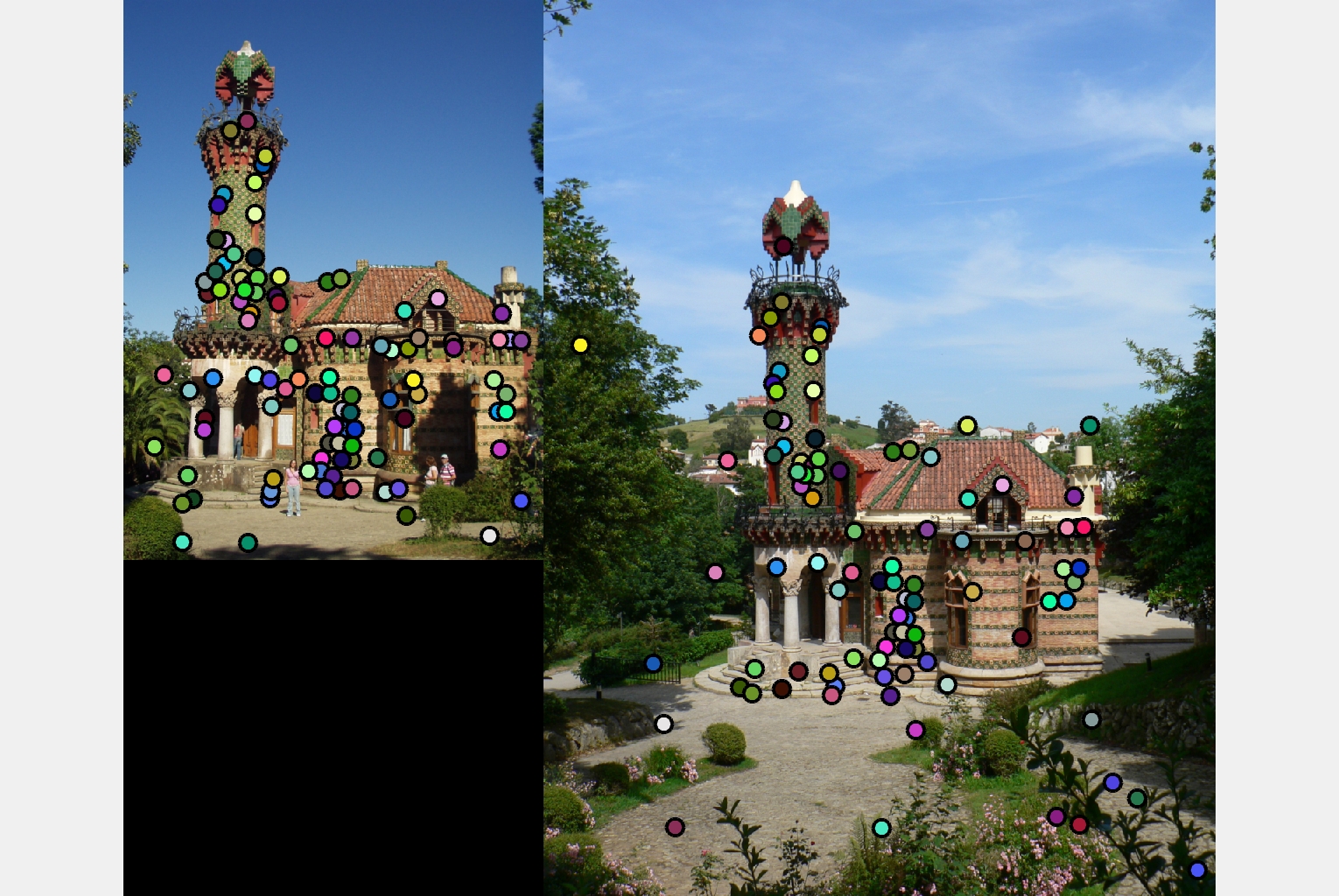
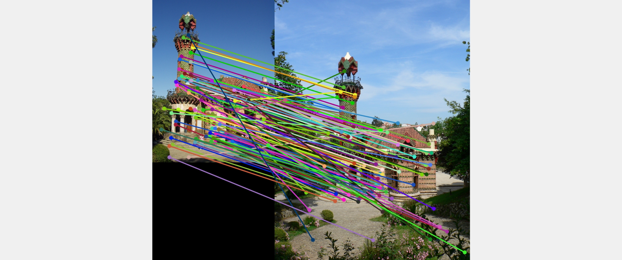
Capricho Gaudi
|
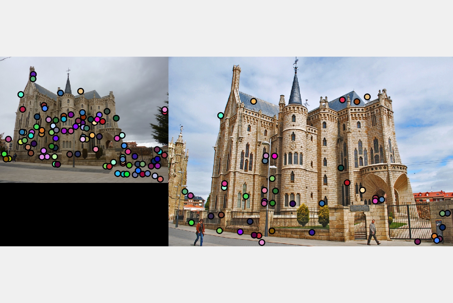
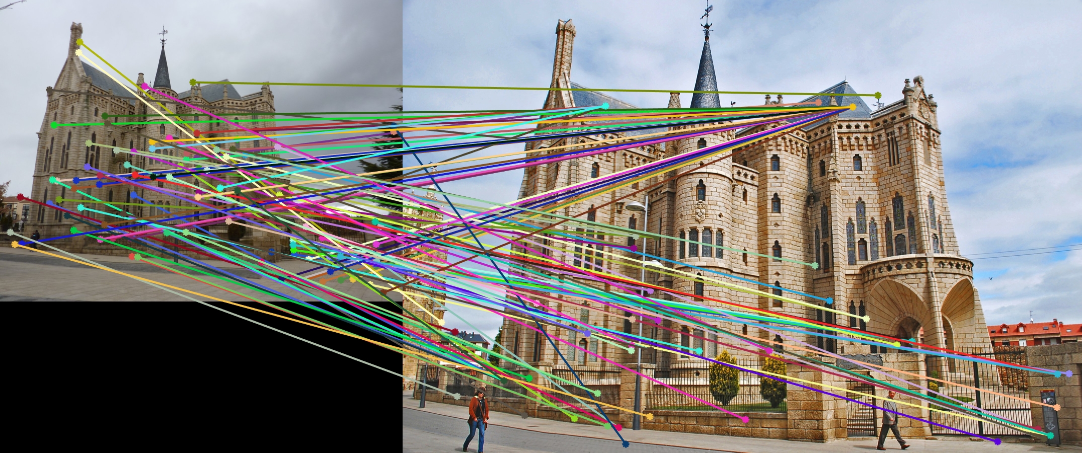
Fig. 14. Although I don't have an exact number for the accuracy of this image, it found many accurate matches.
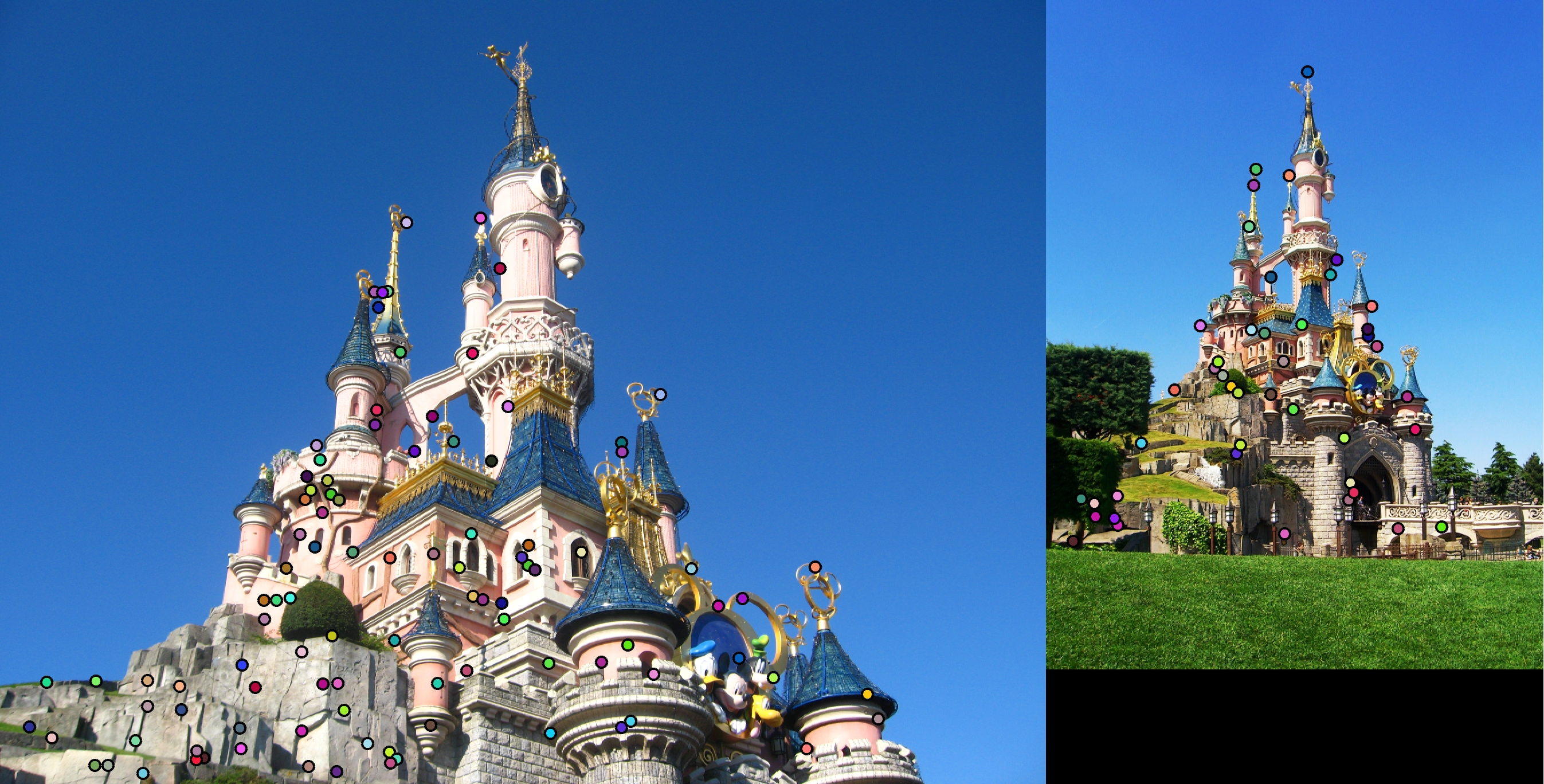
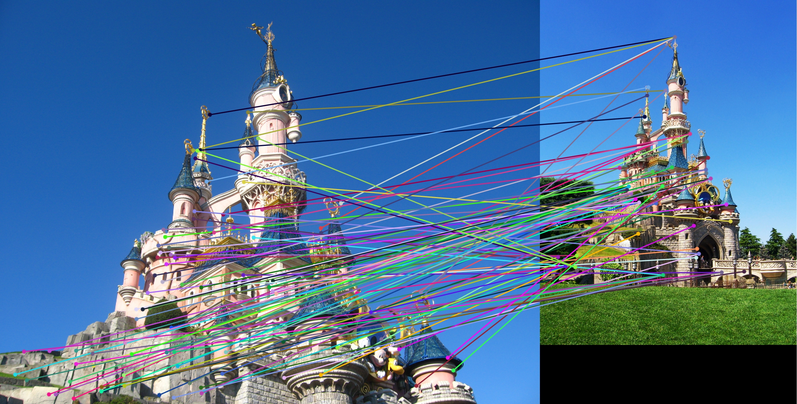
Sleeping Beauty Castle
|
Fig. 15. This wasn't extremely accurate, but it looks like it matched towers decently.