Project 2: Local Feature Matching
Overview
This project consists of implementing the three main parts of a modified SIFT feature detection and feature matching pipeline for images. The pipeline consists of get_interest_points, which finds points of interest in an image, get_features, which gets descriptors for the points of interest, and match_features, which attempts to match descriptors between different images. The purpose of SIFT, or Scale-Invariant Feature Transform, is to be able to robustly and distinctly detect and describe local features in an image so that the features can be reidentified when the algorithm comes across the same feature in a different image, likely with different scale, position, and lighting.
This project was implemented in reverse order of how the pipeline processes the images, as follows:
match_featuresget_featuresget_interest_points
Implementation Details
Matching Features
The function match_features takes two matrices of feature descriptors, features1 and features2, and returns two matrices containing match indices and match confidence values.
    % Get the distances
    dists = pdist2(features1, features2, 'euclidean');

    % Sort by distance
    [dists, indices] = sort(dists, 2);

    % Calculate the confidence values by taking best[2] / best[1]
    confidences = dists(:, 2) ./ dists(:, 1);

    matches = zeros(size(confidences, 1), 2);
    matches(:, 1) = 1:size(confidences, 1);
    matches(:, 2) = indices(:, 1);


    % Sort the matches so that the most confident onces are at the top of the
    % list. You should probably not delete this, so that the evaluation
    % functions can be run on the top matches easily.
    [confidences, ind] = sort(confidences, 'descend');
    matches = matches(ind,:);
The main functionality of matching is taken care of by 2 MATLAB functions: pdist2 and sort. pdist2 calculates the distance between all vectors in features1 and features2, and then, sort sorts each vector descending by distance. Finally, the last major step is calculating the confidence per match, which is accomplished by dividing the second best match by the best match.
Extracting and Describing Features
The function get_features takes in an image, a set of points of interest, and a specified feature_width.
function [features] = get_features(image, x, y, feature_width)

    % Make sure x and y have the same number of features
    assert(size(x, 1) == size(y, 1), 'x and y must have the same number of points');

    if size(image, 3) == 3
        image = rgb2gray(image);
    end

    % Determine the value to clip values to in descriptor
    clip = Inf(1);

    % The number of bins to use
    bin_count = 8;
    assert(mod(bin_count, 2) == 0, 'Bin count must be even!');

    % Calculate values
    cell_width = feature_width / 4;
    offset = feature_width / 2;

    npoints = size(x, 1);

    % Find gradients at each pixel point
    [Gmag, Gdir] = imgradient(image);

    features = zeros(npoints, feature_width * bin_count);
    bins = bin_gradients(Gdir, bin_count);

    for i = 1:npoints
        min_x = x(i) - offset + 1;
        min_y = y(i) - offset + 1;
        max_x = x(i) + offset;
        max_y = y(i) + offset;

        % Check if point is within bounds
        if min_x > 0 && max_x <= size(bins, 2) && ...
                min_y > 0 && max_y <= size(bins, 1)
            Fbins = bins(min_y:max_y, min_x:max_x, :);
            Fmags = Gmag(min_y:max_y, min_x:max_x, :);
            features(i, :) = create_descriptor(Fbins, Fmags, cell_width, bin_count, clip);
        end
    end
end
The main functionality of feature extraction and description is split into two helper functions: bin_gradients and create_descriptor.
bin_gradients is called first, in the line bins = bin_gradients(Gdir, bin_count);, which takes gradient directions of the image and classifies each pixel's direction in one of the bin_count buckets.
function bins = bin_gradients(dirs, bin_count)
    bin_range = (180 - (-180)) / bin_count;
    bin_offset = bin_count / 2 + 1;

    y_size = size(dirs, 1);
    x_size = size(dirs, 2);
    bins = zeros(size(dirs, 1), size(dirs, 2), bin_count);

    for y = 1:y_size
        for x = 1:x_size
            bins(y, x) = floor(dirs(y, x) / bin_range + bin_offset);
        end
    end
end
create_descriptor is then invoked for every interest point, and given the previously created bin assignments for every pixel, the function creates a Histogram of Orientations (HoG) descriptor for each respective interest point.
function descriptor = create_descriptor(bins, mags, cell_width, bin_count, clip)
    descriptor = zeros(cell_width * 4, bin_count);
    desc_index = 1;

    for y = 1:cell_width:size(bins, 1)
        for x = 1:cell_width:size(bins, 2)
            cell_val = zeros(1, bin_count);

            for yy = y:y+cell_width - 1
                for xx = x:x+cell_width - 1
                    cell_val(1, bins(yy, xx)) = cell_val(1, bins(yy, xx)) + mags(yy, xx);
                end
            end

            descriptor(desc_index, :) = cell_val;
            desc_index = desc_index + 1;
        end
    end

    % Flatten descriptor
    descriptor = descriptor(:);

    % Normalize vector
    desc_arr_mag = norm(descriptor);
    if desc_arr_mag > 0
        descriptor = descriptor / desc_arr_mag;
    end

    % Clamp values to [0, clip] if clip is not infinite
    if clip < Inf(1)
        for i = 1:size(descriptor, 1)
            descriptor(i) = min(descriptor(i), clip);
        end
    end

    descriptor = rot90(descriptor);
end
Finding Points of Interest
To detect interest points, the get_interest_points function uses the Harris corner detection algorithm to highlight possible high delta gradient areas (called corners). The function creates a Gaussian filter and builds the Ix, Iy, Ixx, Iyy, and Ixy matrices using imfilter. The function also contains several key, tweakable parameters: nonmax_suppress, whether to enable non-maximum suppression (addressed later), alpha of the Harris algorithm, sigma of the Gaussian used, and gauss_size, the size of the Gaussian used.
function [x, y, confidence, scale, orientation] = get_interest_points(image, feature_width)
    nonmax_suppress = true;
    alpha = 0.08;
    sigma = 2;
    gauss_size = 25;

    if size(image, 3) == 3
        image = rgb2gray(image);
    end

    gaussian = fspecial('Gaussian', gauss_size, sigma);

    [Ix, Iy] = imgradientxy(image);
    Ixx = imfilter(Ix.^2, gaussian);
    Iyy = imfilter(Iy.^2, gaussian);
    Ixy = imfilter(Ix .* Iy, gaussian);

    % Create Harris corners matrix
    H = Ixx .* Iyy - Ixy.^4 - alpha * (Ixx + Iyy).^2;

    % Supress features along the edges
    H([1:feature_width, end - feature_width + (1:feature_width)], :) = 0;
    H(:, [1:feature_width, end - feature_width + (1:feature_width)]) = 0;
    H([1:feature_width, end - feature_width + (1:feature_width)], :) = 0;
    H(:, [1:feature_width, end - feature_width + (1:feature_width)]) = 0;

    % Find corners above adaptive threshold
    threshold = mean2(H);
    H = H .* (H > threshold * max(max(H)));

    % Apply non-maximum suppression using a 3x3 sliding window
    if nonmax_suppress == true
        filter = colfilt(H, [3 3], 'sliding', @max);
        H = H .* (H == filter);
    end

    [y, x] = find(H);
end
Results
Initial Results (Cheat Points)
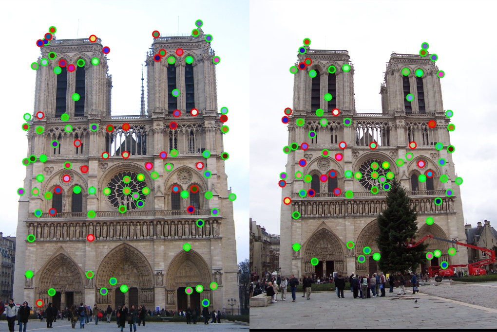
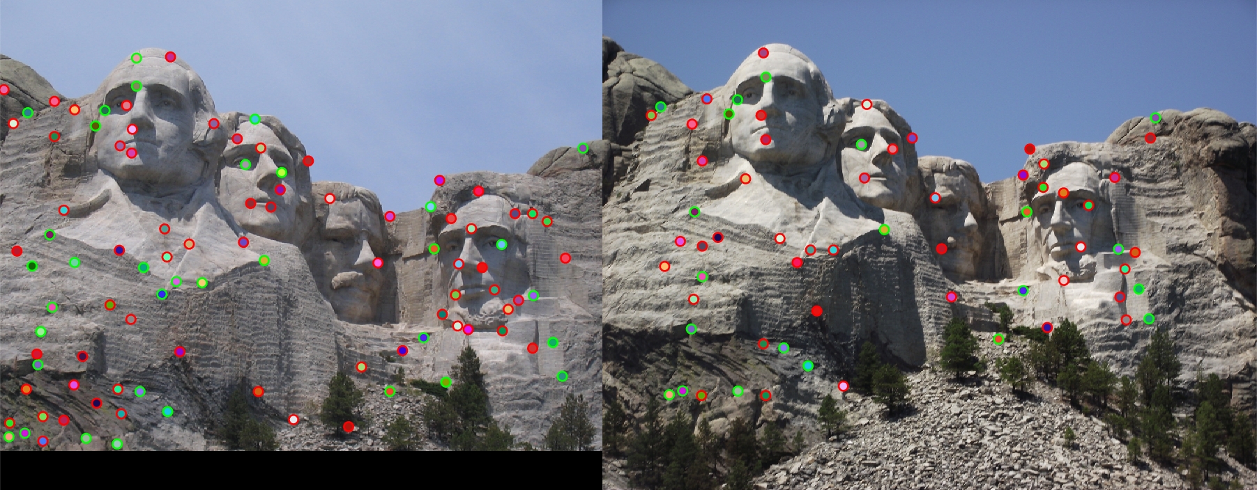
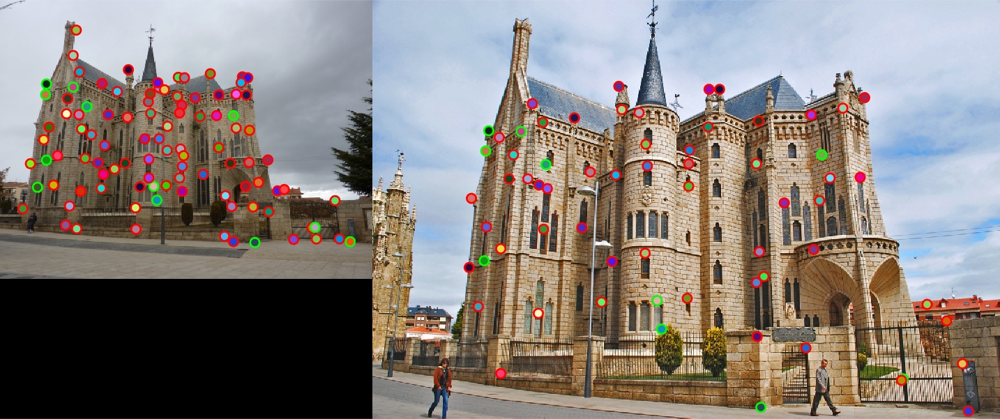
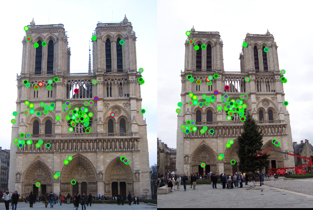
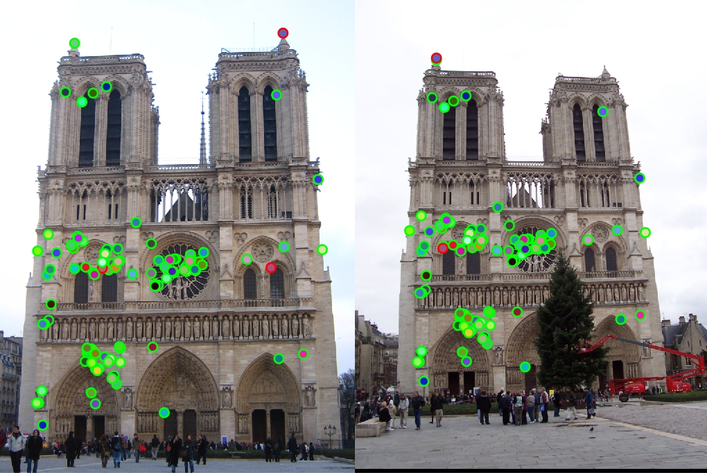
Before even implementing get_interest_points, the function cheat_interest_points gives a baseline for performance of feature description and keypoint matching.
|
|

|
As illustrated by the results above, especially the arrows images, it is clear that the baseline accuracy is quite low. The accuracies for the image sets were as follows: Notre Dame at 55.7%, Mount Roushmore at 28.57%, and Episcopal Gaudi at 9.52%.
This may be due to many factors, some of which include the fact that "cheat" (semi-random) points were used, all matches were considered, regardless of the confidence, and an untuned feature width.
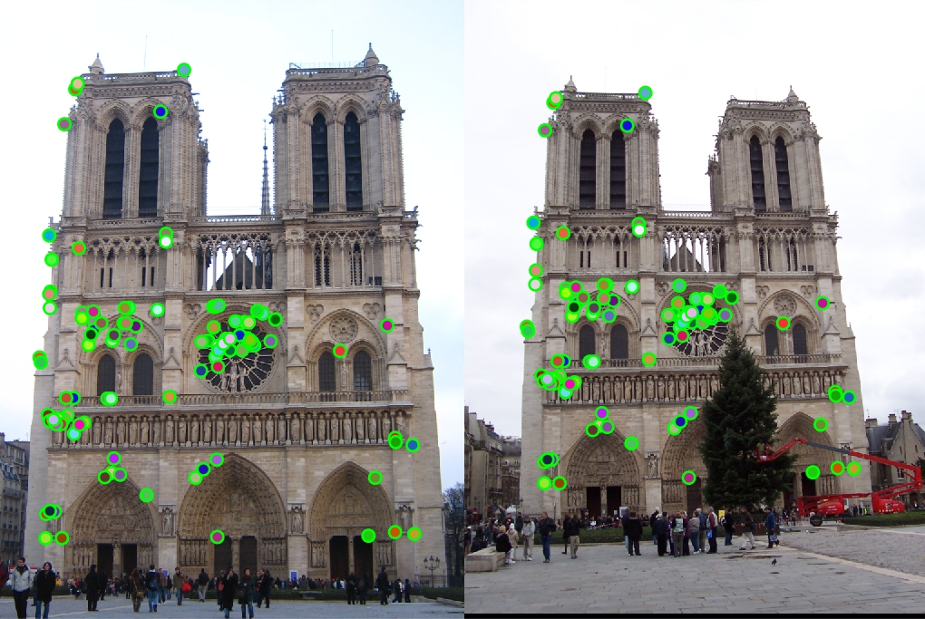
Top 100 Trimming (Cheat Points)
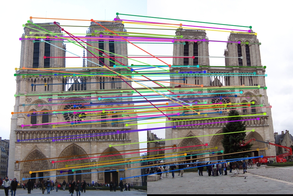
One of the first improvements made to matching was to take the top 100 matches instead of considering all points, and even on the baseline, there was a significant improvement. This was likely due to the fact that some of the matches had low confidence values, which can result in a false match. A low confidence value indicates that the 'best' match and the 'second best' matches had similar distances, so there is more possibility for an error in the match.
|
|
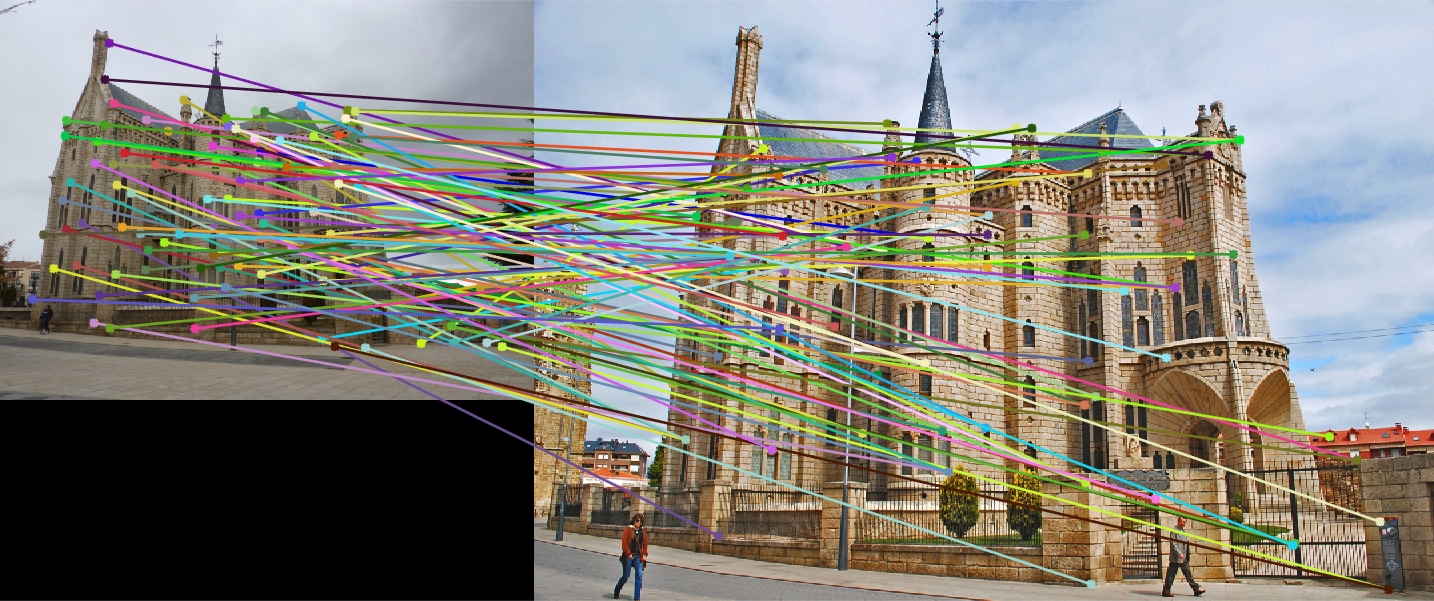
|
The accuracy of the keypoint matching jumped up to the following values: Notre Dame at 68.0%, Mount Roushmore at 35.0%, and Episcopal Gaudi at 12.0%.
Introducing get_interest_points
Bonus: Non-Maximum Suppression
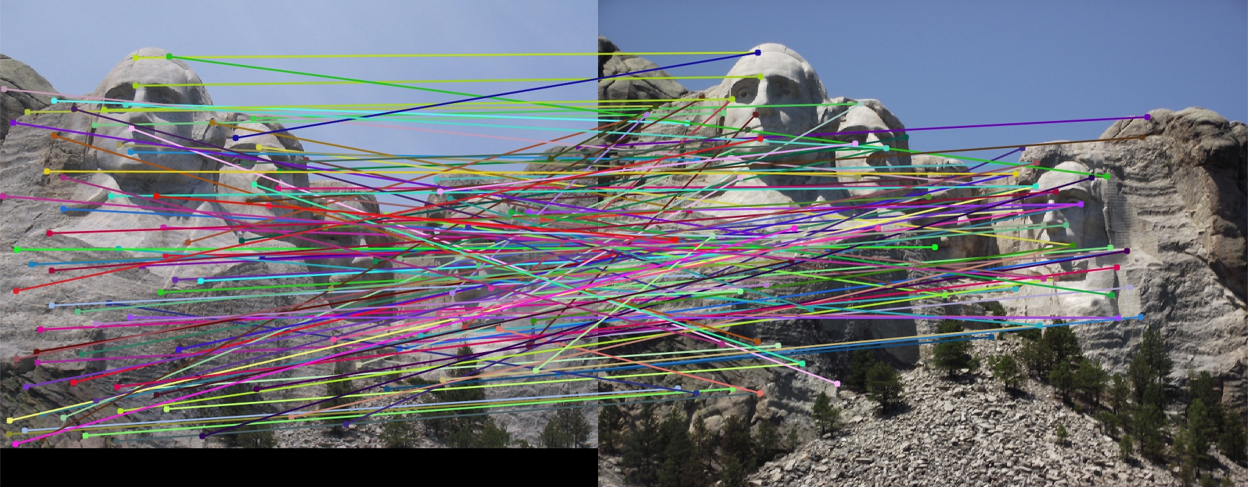
The second optimization that was implemented early on (and turned out to be a bonus) was non-maximum suppression, which helped both in interest point detection and computation performance. Non-maximum suppression takes a sliding window across the corners detected during the get_interest_points step and within that window, removes any corners detected within that window that are not the maximum corner. This helps reduce the number of redundant points of interest detected by Harris corners. Interestingly, the pipeline refused to run without non-maximum suppression, erroring out because the requested array during the matching step would exceed 42 GB/74 GB (depending on the image set) in memory (due to pdist2). By incorporating non-maximum suppression, the number of interest points found were reduced by almost tenfold for the Mount Rushmore image set. Because of these major improvements, especially in computation performance, non-maximum suppression is used for the remainder of the results described.
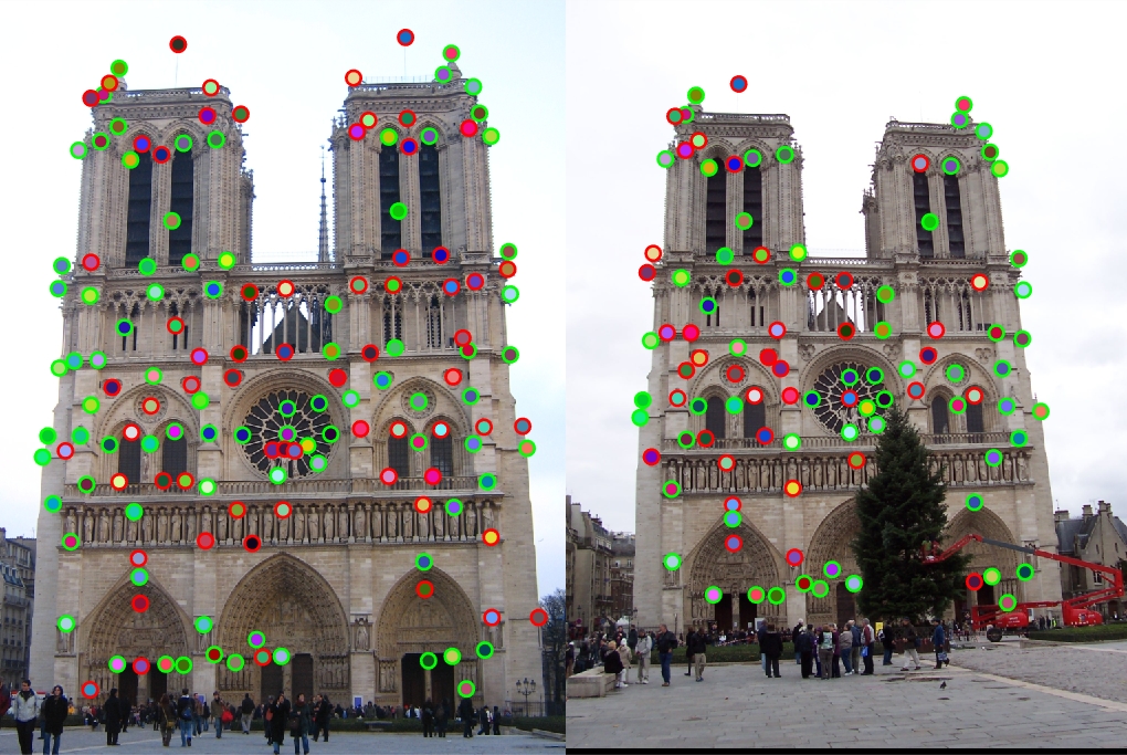
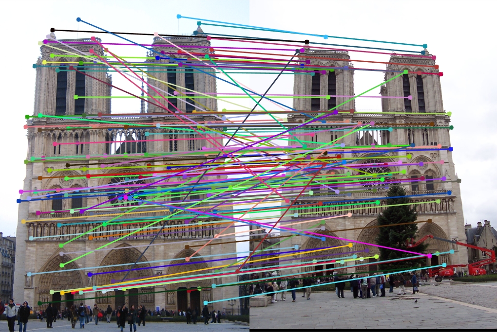
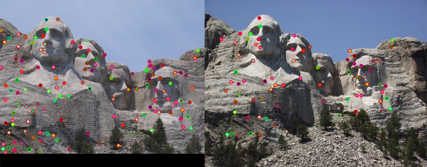
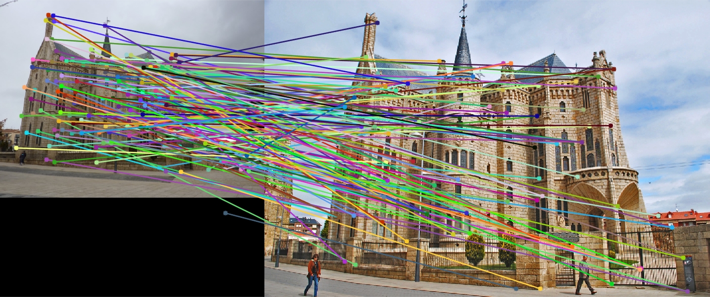
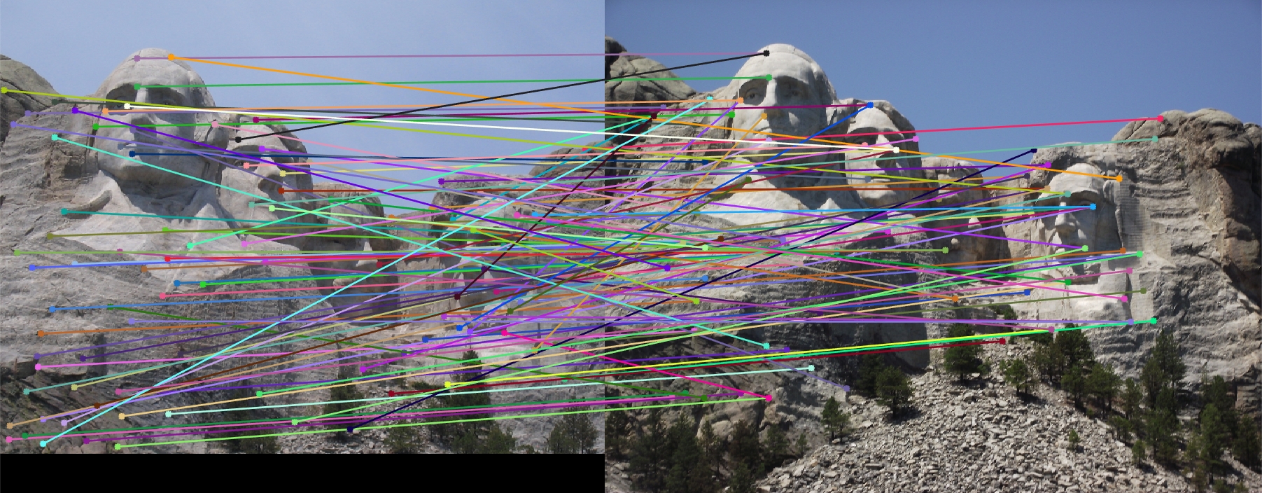
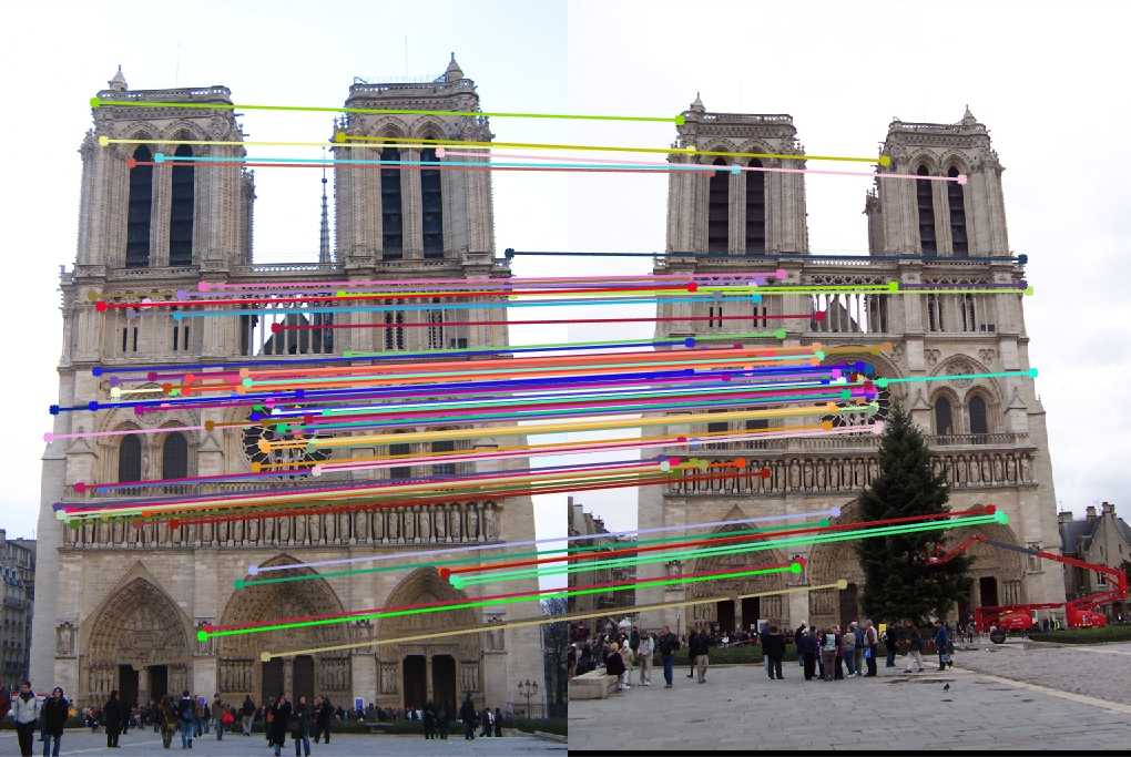
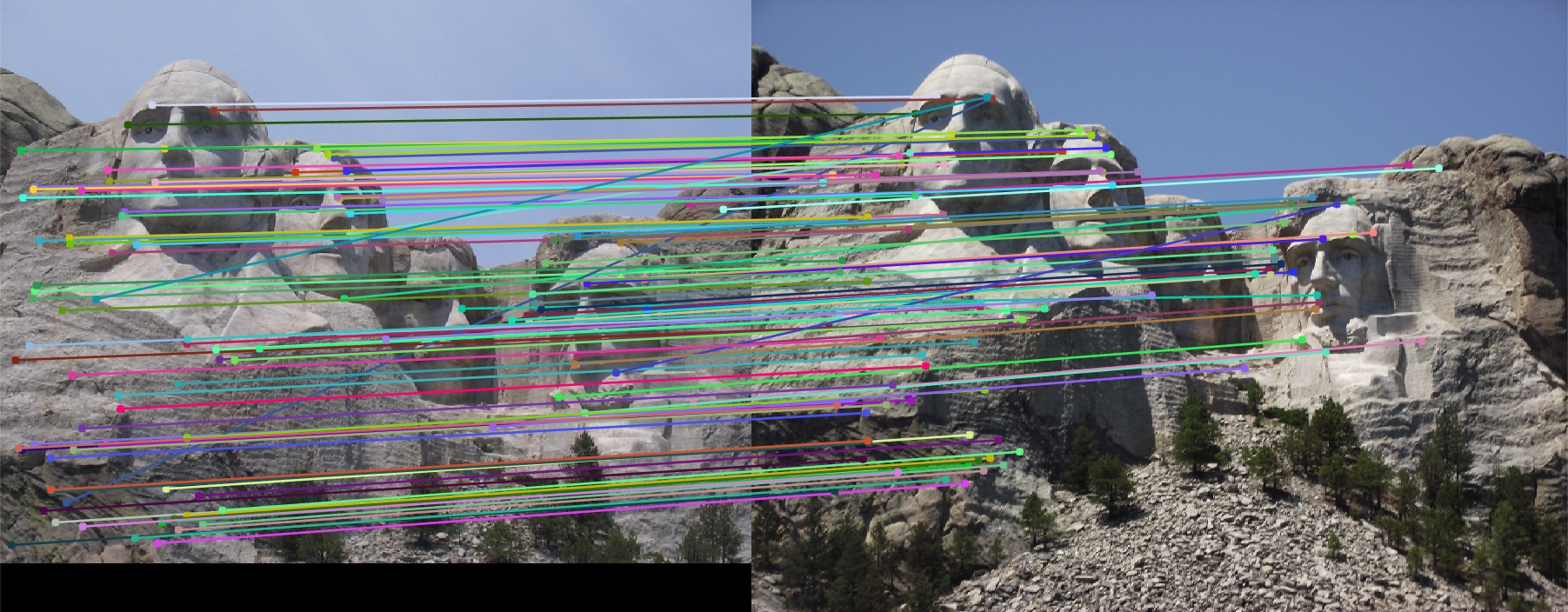
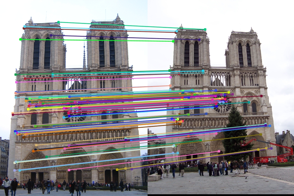
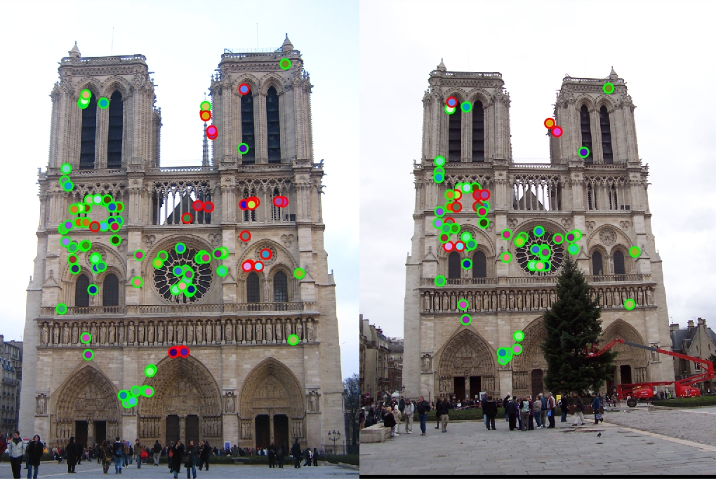
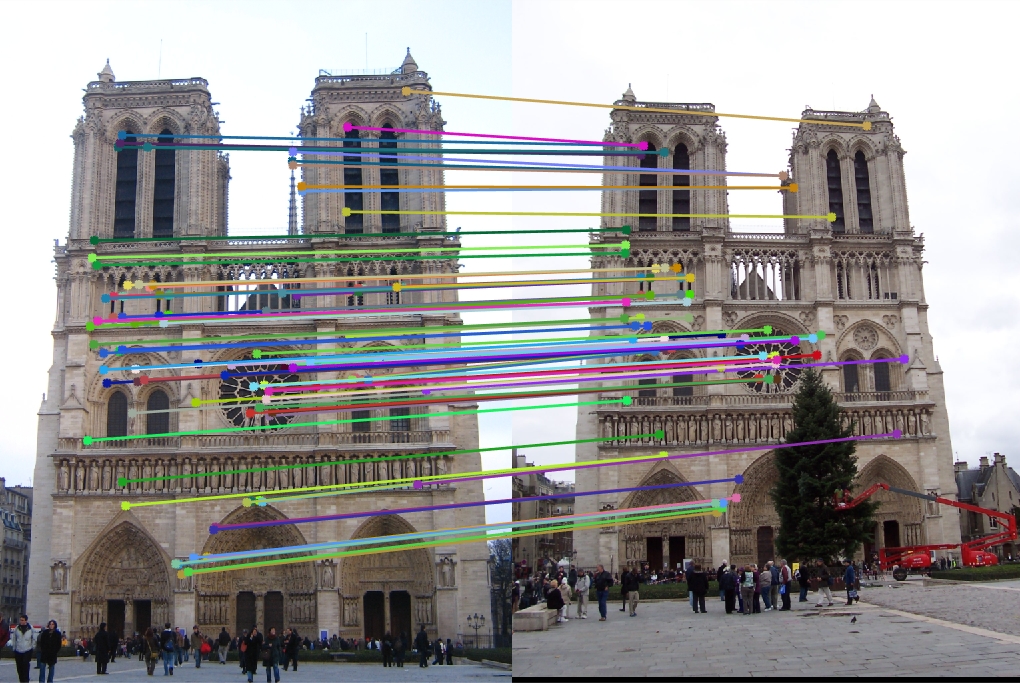
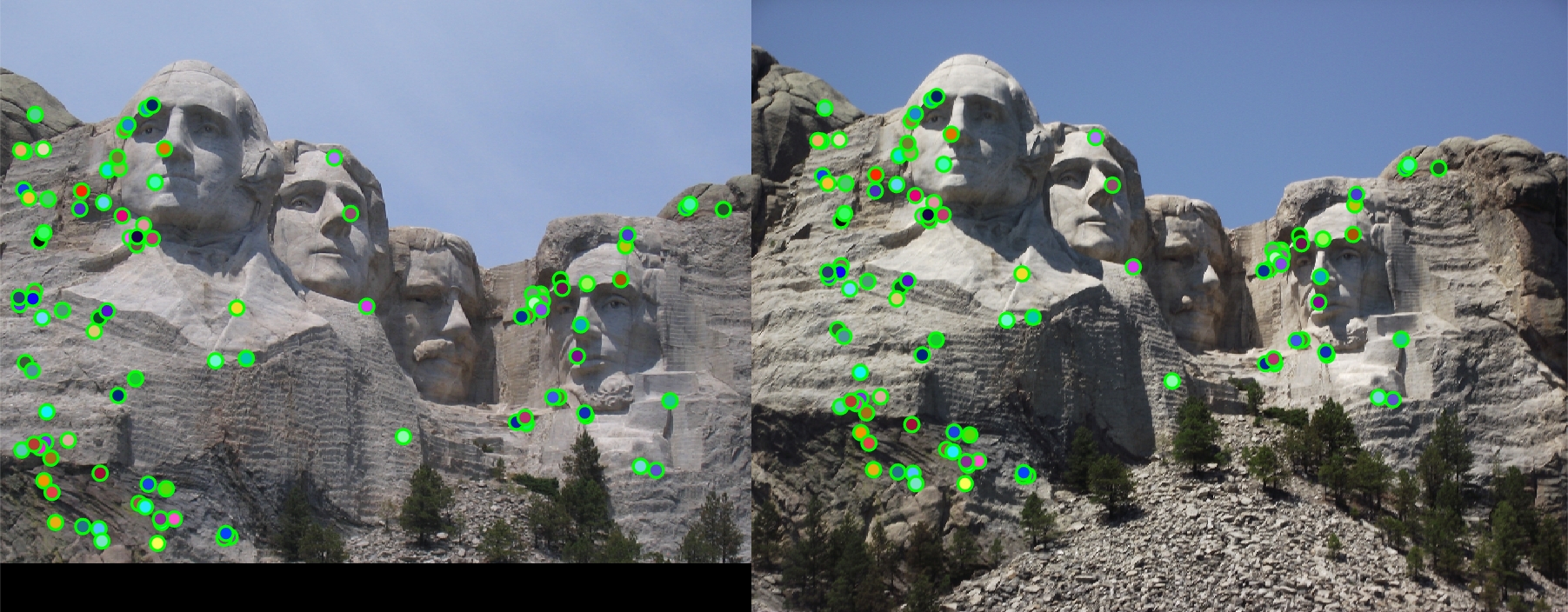
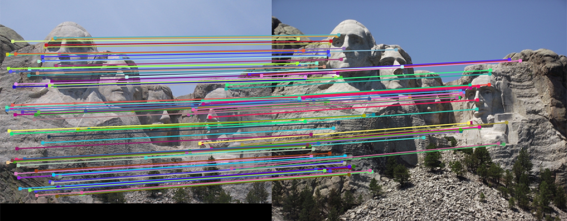
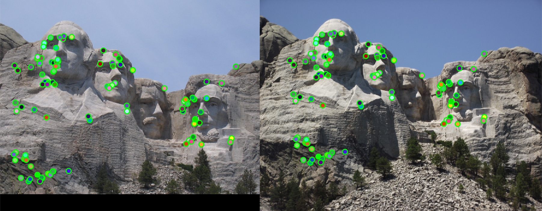
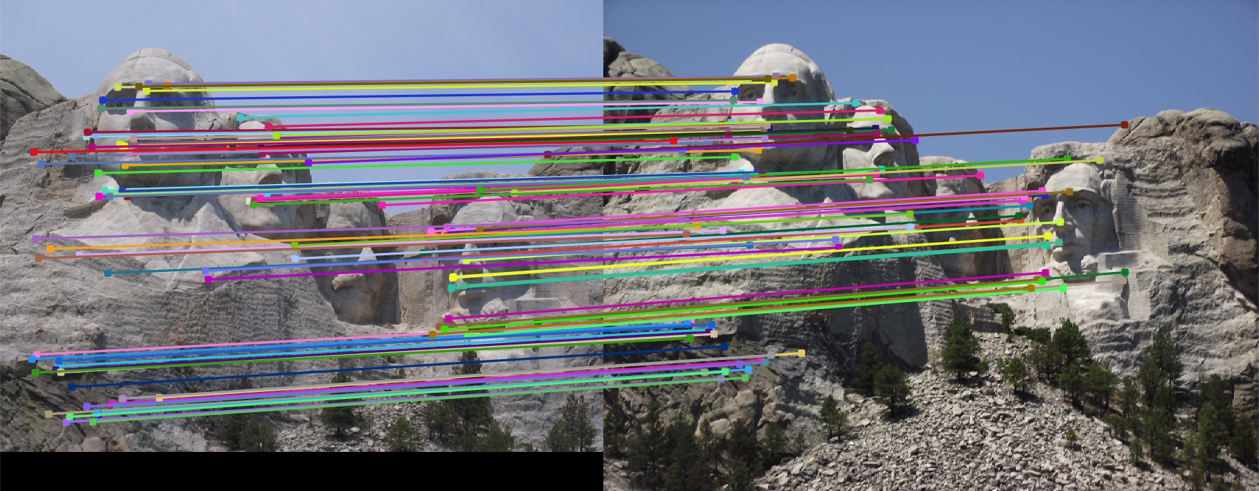
To replace the cheat points, the get_interest_points function was used to identify actual points of interest, and the results for every image set improved greatly. This can be explained by the fact that the points detected are a lot more unique, being at areas of high gradient change (corners).
|

|
|
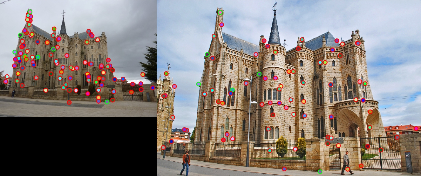
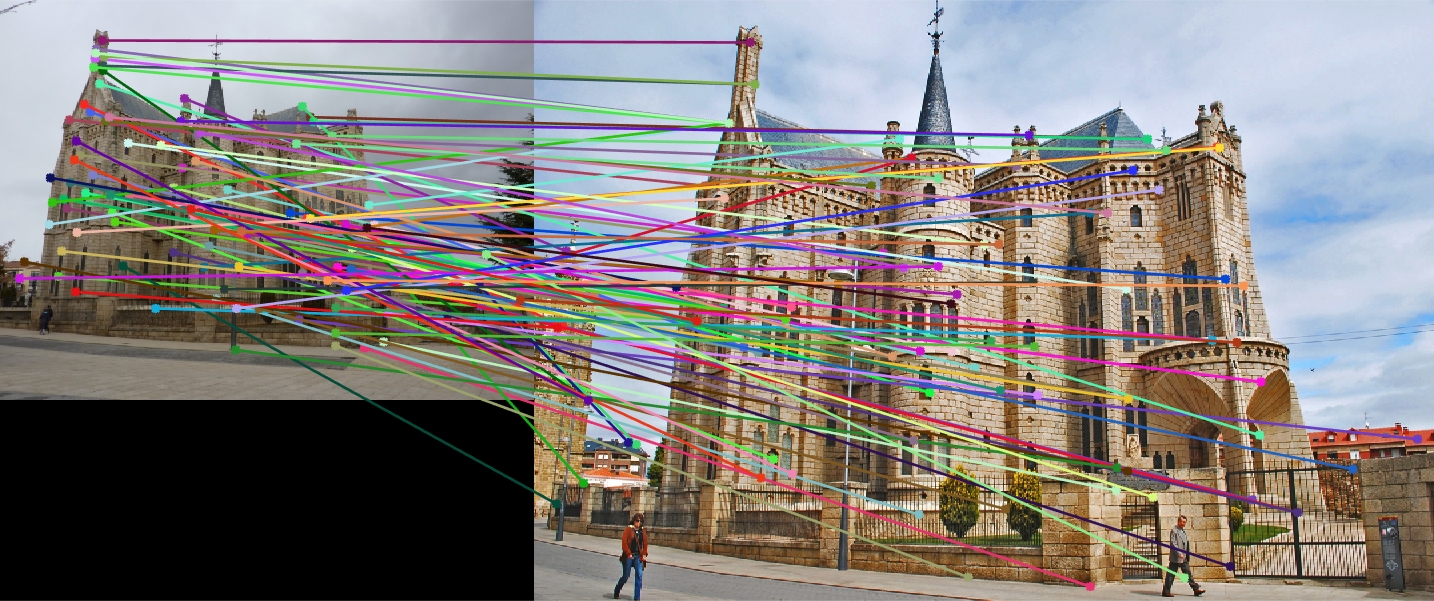
Again, the accuracies illustrate the algorithmic improvement perfectly. Compared to the cheat points, Notre Dame is up to 96.0% from 68.0%, Mount Roushmore is up to 93.0% from 35.0%, and Episcopal Gaudi down to 8.0% from 12.0%. Interestingly, the Episcopal Gaudi keypoint matching degraded in performance compared to the baseline, and with tweaking (below), the performance of SIFT on the image set improves.
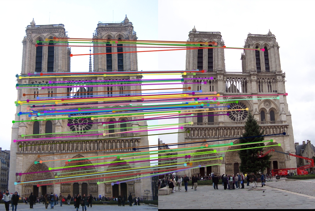
Bonus: Parameter Tweaking
One of the most impactful parameters that is modifiable is the feature_width variable in proj2.m. This parameter adjusts the size of the feature descriptor blocks created by the get_features function. Changing this value can have a serious impact on keypoint matching accuracy since it fundamentally modifies the range of the neighborhood the algorithm describes as part of the keypoint.
Notre Dame

|
|

|
|
Accuracy Values
16x16 Features:
96 total good matches, 4 total bad matches.  96.00% accuracy

32x32 Features:
100 total good matches, 0 total bad matches.  100.00% accuracy

64x64 Features:
88 total good matches, 12 total bad matches.  88.00% accuracy

128x128 Features:
73 total good matches, 27 total bad matches.  73.00% accuracy
The Notre Dame image set benefitted from smaller feature descriptors, although it is evident that the algorithm still benefits a little from slightly more neighboring pixels accounted for in the descriptor (32x32). However, as the size of the features exceeds 64, the accuracy goes down because the larger cell sizes no longer helps (too many neighboring pixels).
Mount Rushmore


|
|
|
|
Accuracy Values
16x16
93 total good matches, 7 total bad matches.  93.00% accuracy

32x32 Features
100 total good matches, 0 total bad matches.  100.00% accuracy

64x64 Features
100 total good matches, 0 total bad matches.  100.00% accuracy

128x128 Features
100 total good matches, 0 total bad matches.  100.00% accuracy
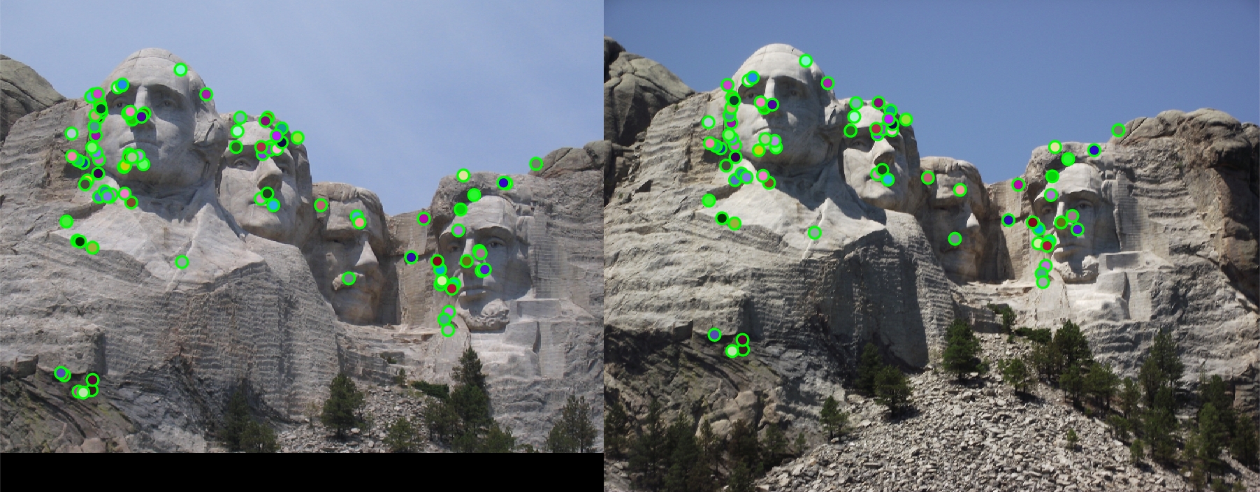
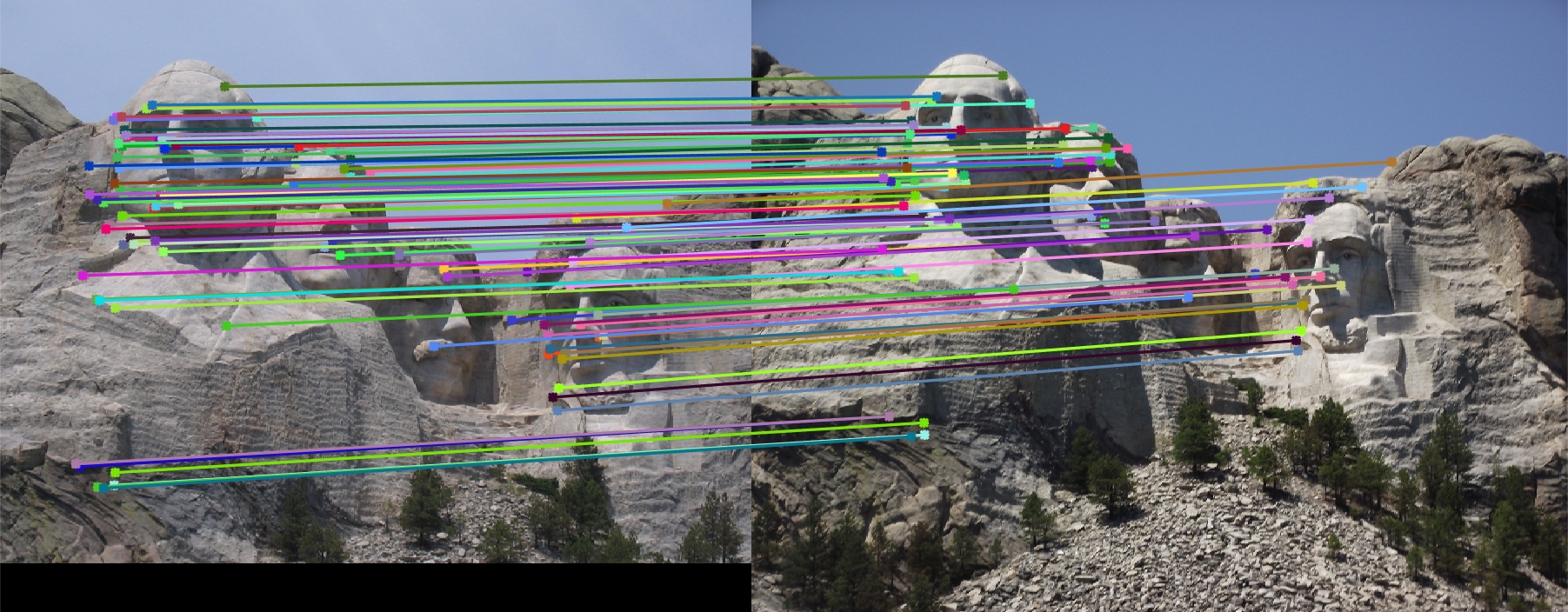
The Mount Rushmore image set clearly benefits from larger feature sizes, and as long as the feature_width is larger than 16, it reaches 100% accuracy. This is surprising considering this image set had the largest contrast difference between the two images, but because the algorithm does well with normalizing values during the get_features step, it does not effect the keypoint matching.
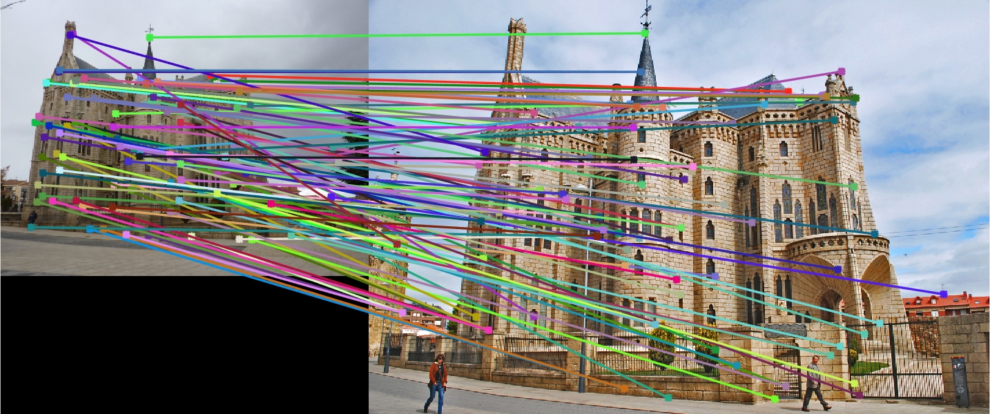
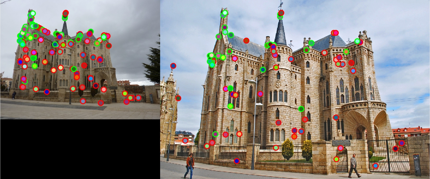
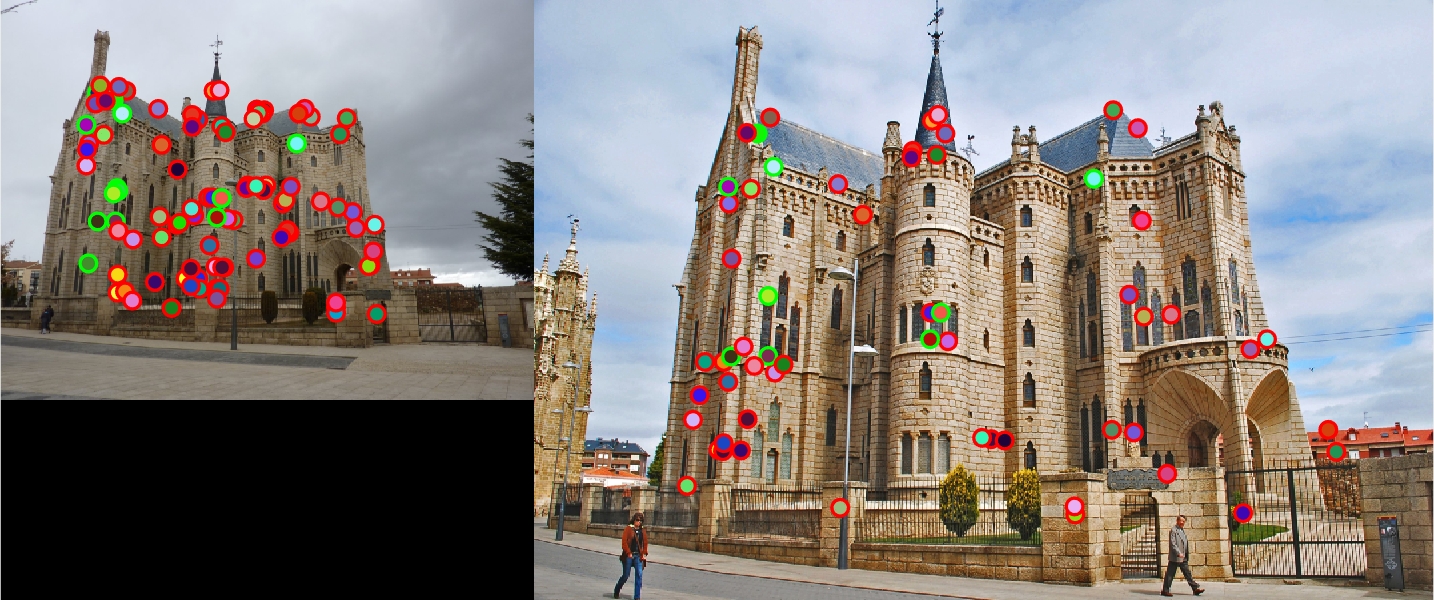
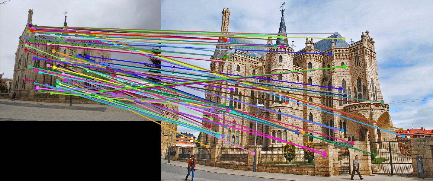
Episcopal Gaudi


|

|

|
|
Accuracy Values
16x16
8 total good matches, 92 total bad matches.  8.00% accuracy

32x32
16 total good matches, 84 total bad matches.  16.00% accuracy

64x64
40 total good matches, 60 total bad matches.  40.00% accuracy

128x128
15 total good matches, 85 total bad matches.  15.00% accuracy
The impact of the feature_width is perhaps best seen by the Episcopal Gaudi image set. There is a clear sweet spot around 64x64, which is a perfect balance between the tradeoffs of specifity and local context for the descriptor.
Histogram Orientations
The parameter for the number of bins (or directions) in the histogram was also experimented with, and the tradeoffs were similar to those of feature_width. Both the Notre Dame and Mount Rushmore image sets match accuracy suffered from modifying the default number of 8 bins. This was unsurprising, since the default parameters were already optimal (100.0% accurate when modifying feature sizes, 32x32 and 64x64 respectively, and using 8 orientations). With the Episcopal Gaudi image set, increasing the bin value from 8 to 12 made minimal difference, increasing accuracy by a meager 1.0% (up to 41.0%), which is more likely noise than actual improvement.