Project 2: Local Feature Matching
Example of a hybrid image.
The goal of this project is to create a local feature matching algorithm using techniques described in Szeliski chapter 4.1. The pipeline is a simplified version of the famous SIFT pipeline. The matching pipeline is intended to work for instance-level matching -- multiple views of the same physical scene. There are three key components to the pipeline: interest point detection, local feature description, and feature matching.
Interest point detection
To find interest points I implemented the Harris corner detector. First, I blurred the image with a Gaussian filter to remove high frequency variations. Next, I computed the gradients in the x and y direction using a Sobel filter. Then, I filtered Ix^2, Ix.*Iy, etc with gaussians to obtain the necessary terms for the Harris function. Lastly, I computed the Harris function values at every pixel. I threw out points whose Harris value was lower than a threshold. Then I performed nonmaximal supression by simply finding points which were higher than all their neighbors. This gave me a list of interest points with high Harris corner function values. I passed on 3000 points which had the highest Harris scores.
Local feature description
For the feature description I used a SIFT-like feature. First, I blurred with image with a Gaussian filter. Next, I calculated the gradient at each pixel with the matlab function imgradient. Then, at each interest point, I performed histogram binning to bin the orientations of nearby pixels. At the interest point, I created a 16x16 grid, and for each pixel in this grid I created 8 bins for 8 different orientations. Each pixel was added to the corresponding orientation bin. Then, in blocks of 4x4, I added up the histograms counts. This gave a final feature count of 4x4x8=128. I also normalized the features to unit length, and I also raised the features to the power of 0.4 to skew the scaling of the features.
Feature Matching
For feature matching I used the ratio test method based on the nearest neighbor distance ration (NNDR) metric. First, given two lists of points, I calculated the distances between the points in the lists. I then considered the list with the least number of features. For each element of this list, I found the closest and the second closest match in the other list (by Euclidean distance). I then recorded the confidence of the match with the closest match as the ratio dist(2nd-best match)/dist(1st-best match). Finally, I found the most confident matches and took the best 100.
Preliminary Results
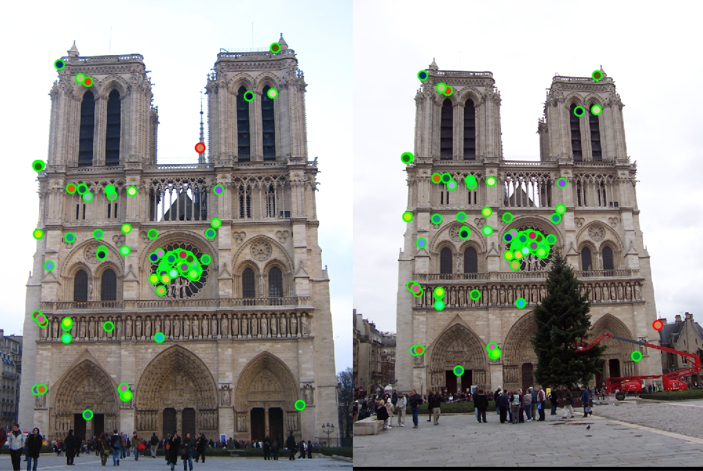
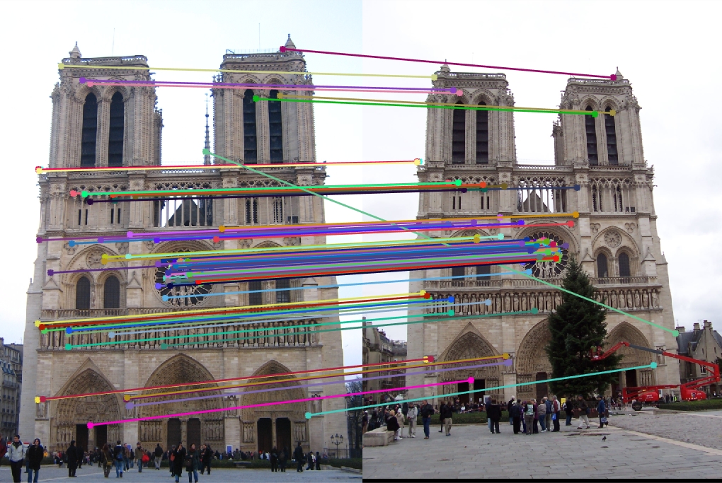
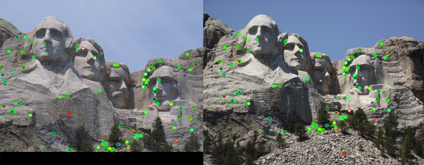
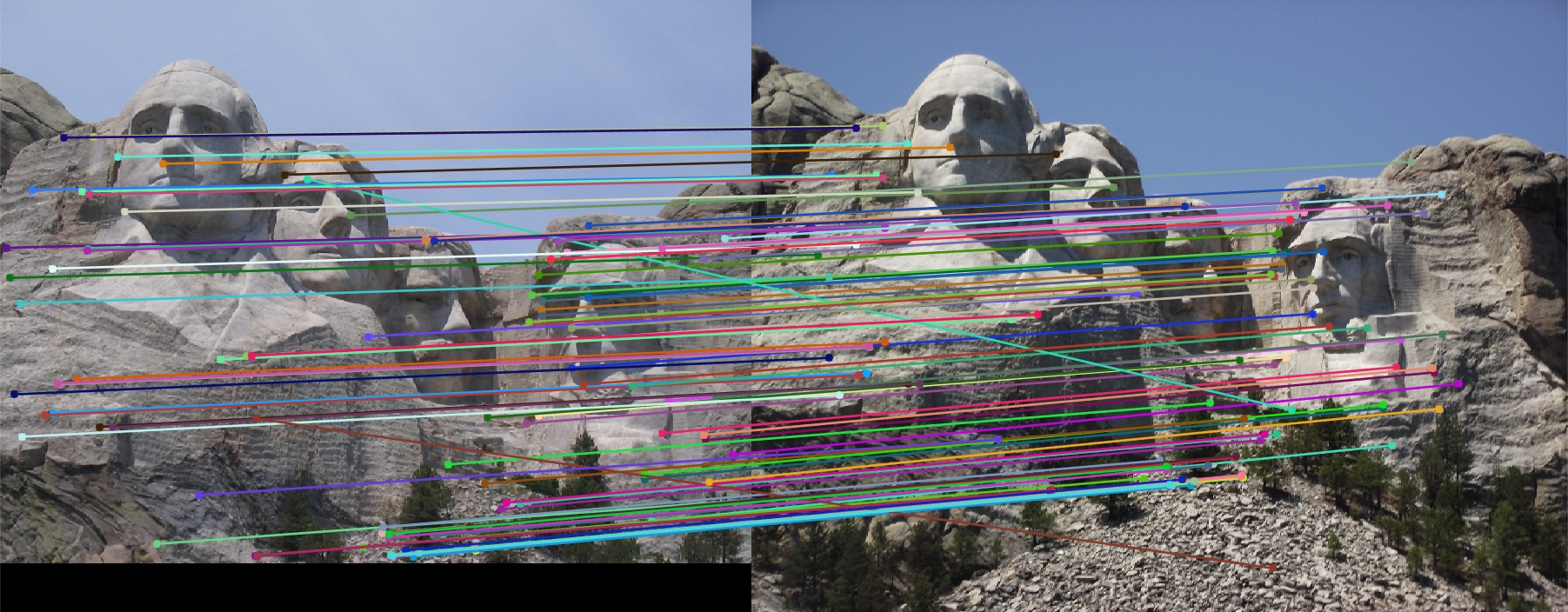
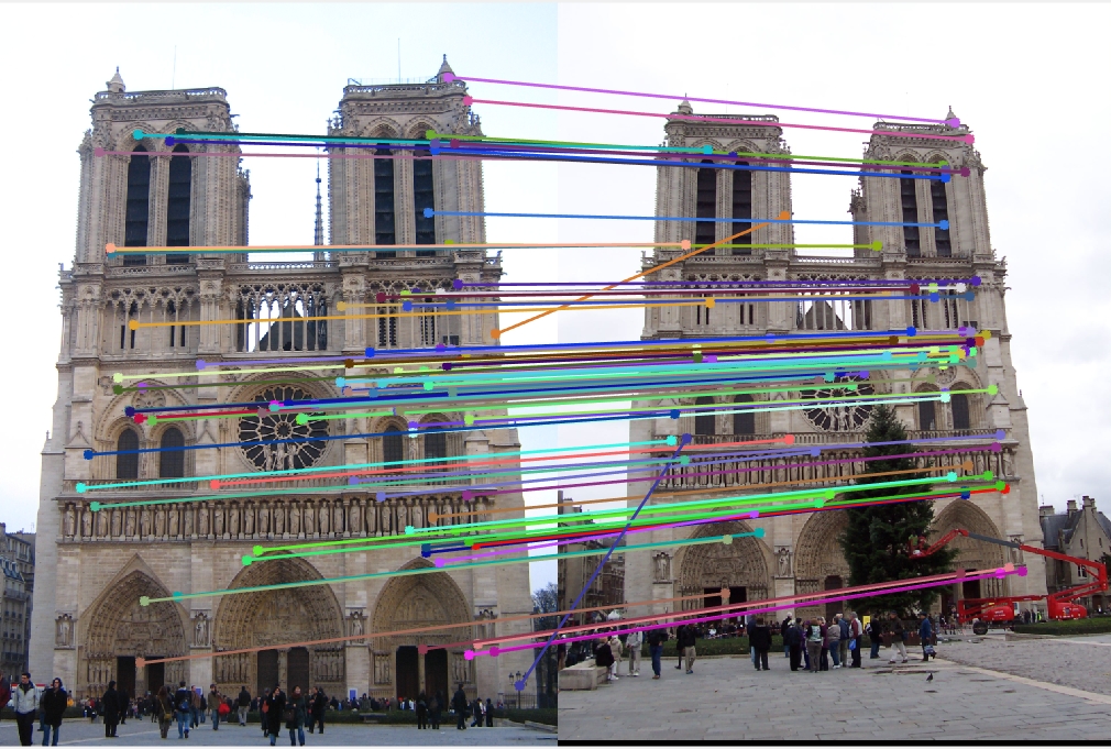
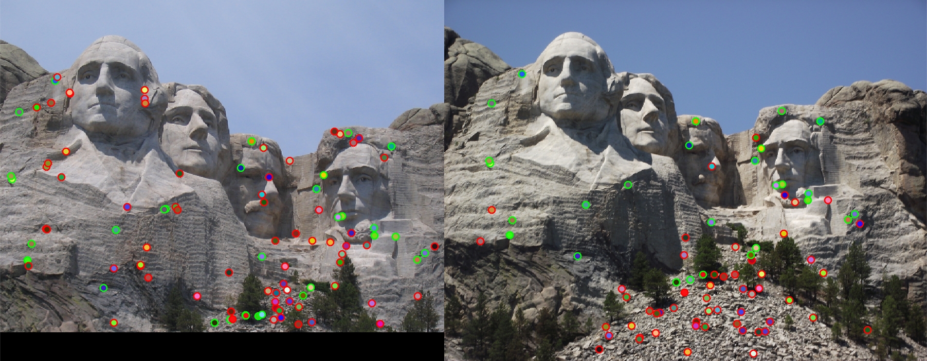
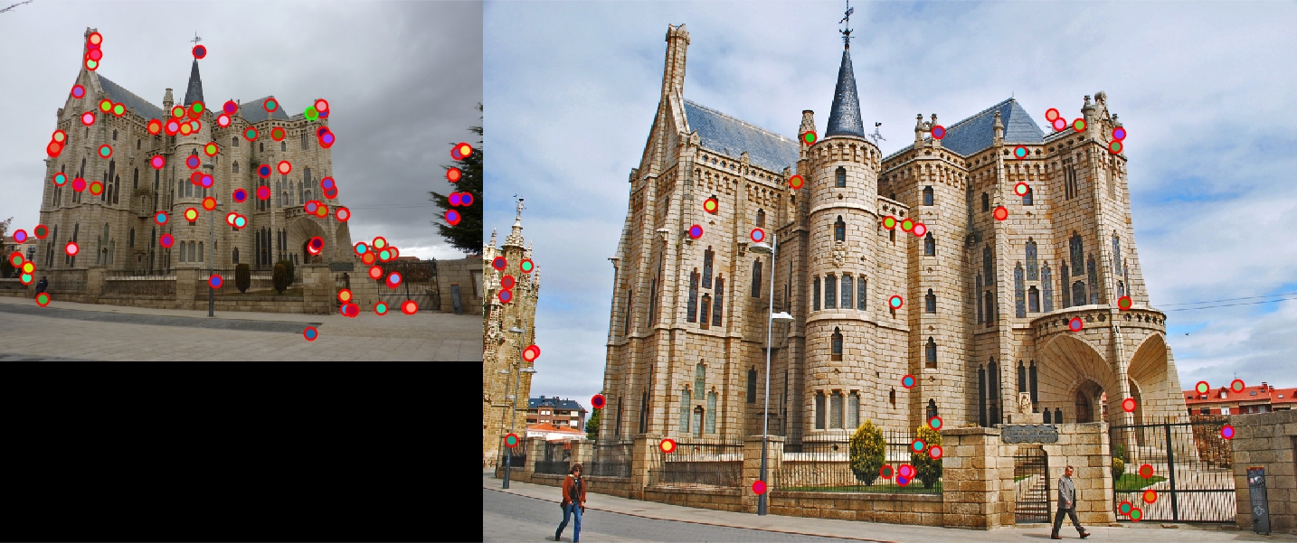
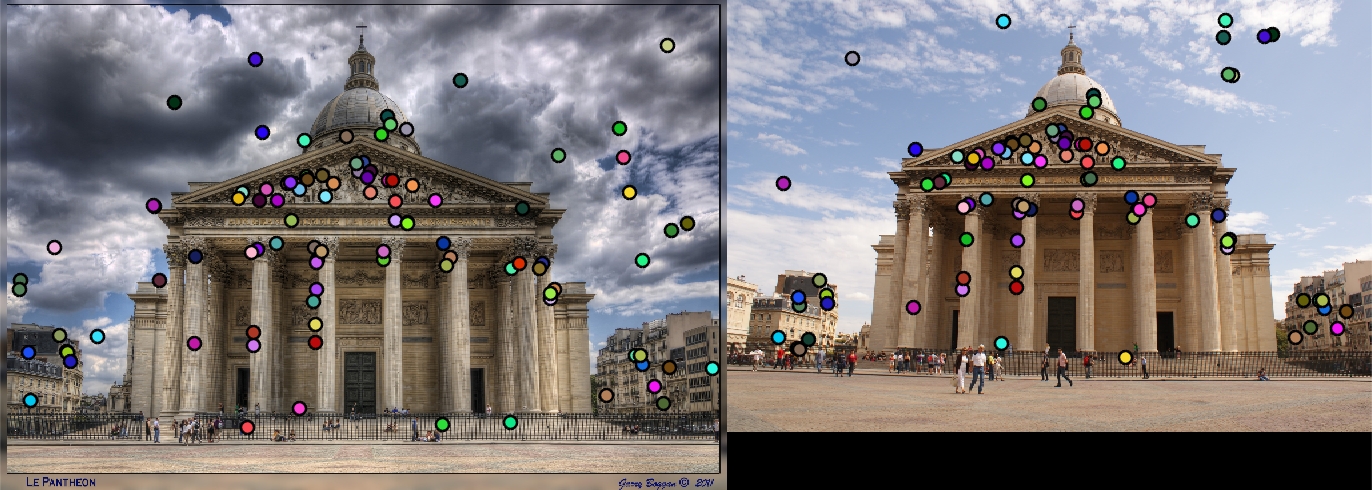
When using cheat_interest_points() instead of my own implementation, I got scores of 76%, 53%, and 14% on the Notre Dame, Mount Rushmore, and Gaudi test pairs, respectively. With the full basic pipeline including Harris corner interest point detection, SIFT-like feature description, and Nearest Neighbor Distance Ratio matching, I was able to achieve scores of 99%, 96%, and 4% accuracy on the three test pairs. Here are the results for those scores:
|
Results for basic pipeline.
While the Notre Dame and Mount Rushmore pairs performed very well, the Gaudi test pair performed very poorly. However, with some parameter tuning (increasing the gaussian blur before finding interest points) I was able to increase the test accuracy to 8%.

|
EXTRA: Scale invariant interest points and features
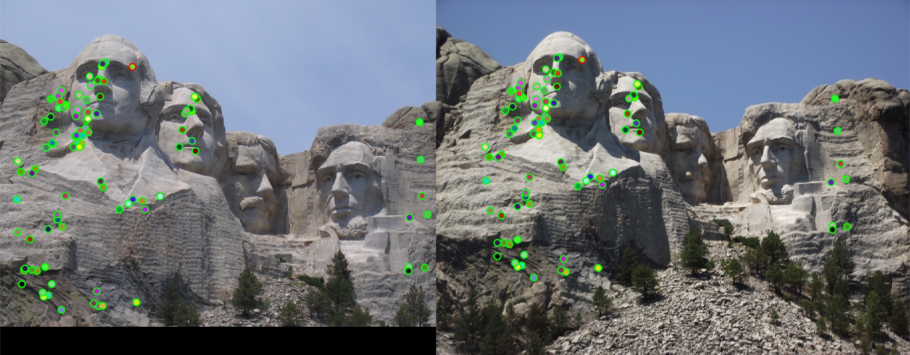
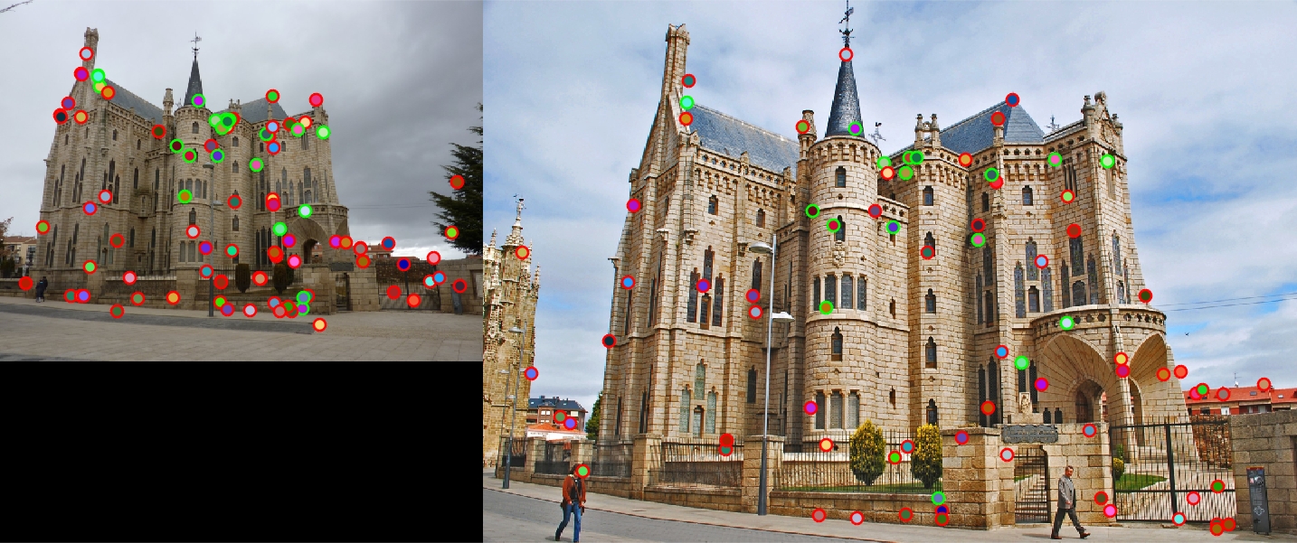
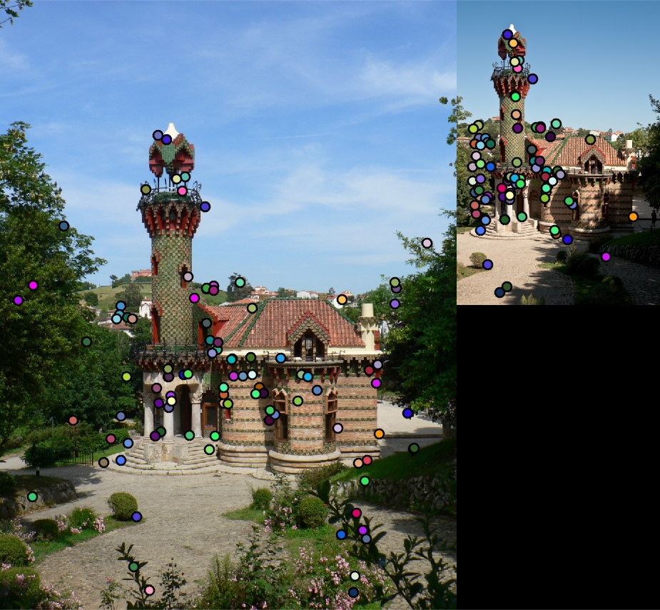
To attempt to handle the scaling problem, especially with the Gaudi image pair, I implemented an automatic scaling detection when finding interest points. I resized the image before calculating the Harris score, then resized it back to original size. Having done this for a range of resize scales, I then picked points which had locally maximal Harris values in both space and scale. I saved the scale at which the maximum Harris value was found; this was the scale of the interest point. Next, when calculating SIFT features, I resized the image to the same scale that the interest point corresponded to in order to create a more scale-invariant feature. With this added to the pipline I achieved scores of 93%, 99%, and 21% accuracy on the Notre Dame, Mount Rushmore, and Gaudi test pairs, respectively. While the Notre Dame image suffers slightly in performance, Mount Rushmore improves a bit and Gaudi improves substantially. This may be due to the fact that the Mount Rushmore images have slight scaling differences and the Gaudi images have strong scaling differences, while the Notre Dame images have less scaling differences to contend with.
|
Results for basic pipeline with automatic scale detection.
EXTRA: Local self-similarity features
I also tried computing feature descriptions using the Local Self-Similarity (LSS) method described in the paper by Shechtman and Irani (CVPR'07) entitled "Matching Local Self-Similarities across Images and Videos". (Details found here: http://www.wisdom.weizmann.ac.il/~vision/SelfSimilarities.html). My implementation was as follows: First, I calculated the sum of square differences (SSD) between patches, where the patch centered at the interest point was compared with patches in a local region surrounding the interest point. Each pixel around the interest point in some local radius was assigned an SSD value. I then took the negative exponent of the SSD to obtain the local correlation surface. I then used a log-polar grid to find the maximal correlation values for each grid location. Finally, after normalizing, these correlation values formed the feature. I was able to achieve scores of 78%, 32, and

|
Results for pipeline with Local Self-Similarity (LSS) features.
EXTRA: PCA reduction of SIFT feature
In order to try to achieve a speed-up when matching features, it is desirable to reduce the dimensionality of the features. The SIFT features I used had a dimension of 128. Using PCA, we can reduce this number of any lower number at the cost of a reduced match rate. To calculate the PCA bases, I took images from the training/validation set of the PASCAL Visual Object Classes dataset (VOC2007, found at http://host.robots.ox.ac.uk/pascal/VOC/voc2007/index.html). The dataset consisted of 5011 color images of a variety of objects and settings. From each image I used the Harris corner detection to find interest points, then I used my SIFT-like feature descriptor to calculate features for each data point. I then used all the features from all the interest points and from all the images to calculate the PCA bases. To do this in a computationally efficient manner, I used the eigen decomposition of the matrix X.'*X, which was 128x128, as follows:
%find principal components of large matrix
[V D]=eig(allfeatures.'*allfeatures);
S=sqrt(D);
where V are the right singular vectors and S is the standard deviations. I was then able to calculate the coefficients of a feature with:
%get PCA coefficients from feature
pca_coeff=feat'*V*S^(-1);
feat=pca_coeff(end-num_pca_feat+1:end);
The last coefficients correspond to the more principal vectors, and are used as the new features. I then calculated the computation time to find the matches and match rate for varying numbers of PCA features on the Notre Dame example.
| # Feat | Match % | Time (s) |
|---|---|---|
| 128 | 96 | 9.39 |
| 64 | 98 | 8.85 |
| 32 | 96 | 7.06 |
| 16 | 88 | 6.8 |
| 8 | 39 | 6.67 |
The conclusion is that it seems that using 32 PCA features results in a hefty speedup while maintaining the same level of matches.
Final Results
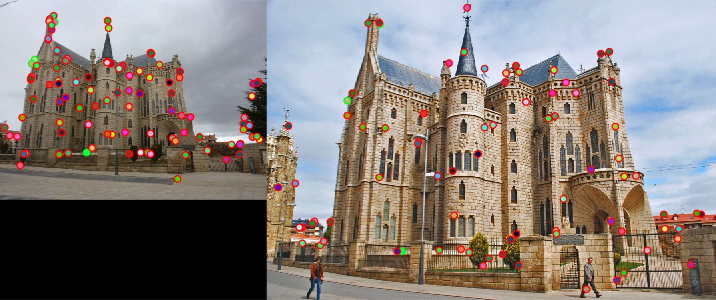
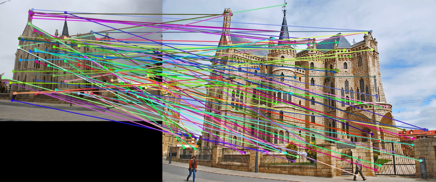
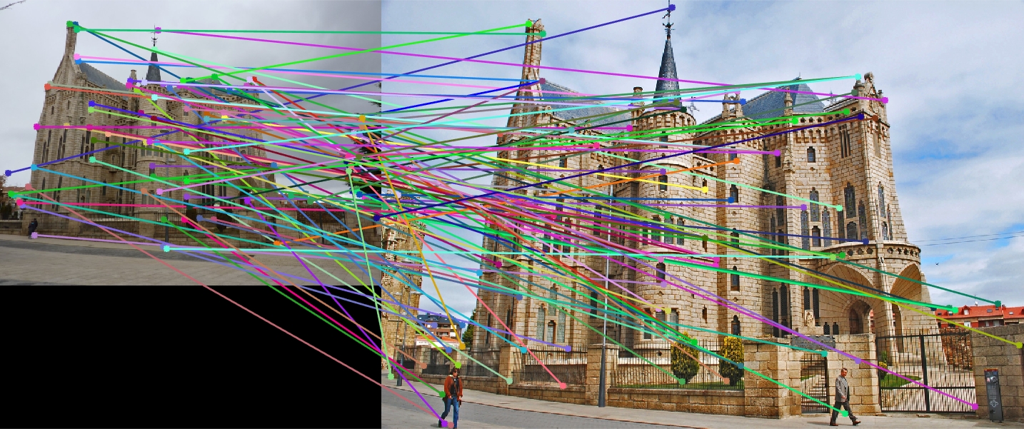
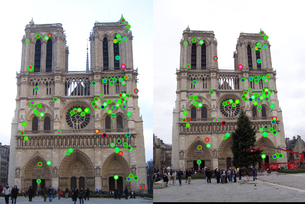
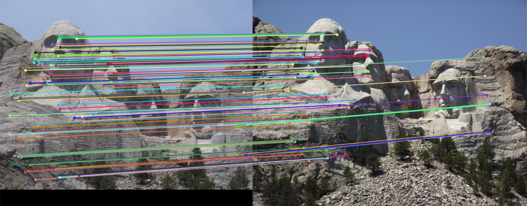
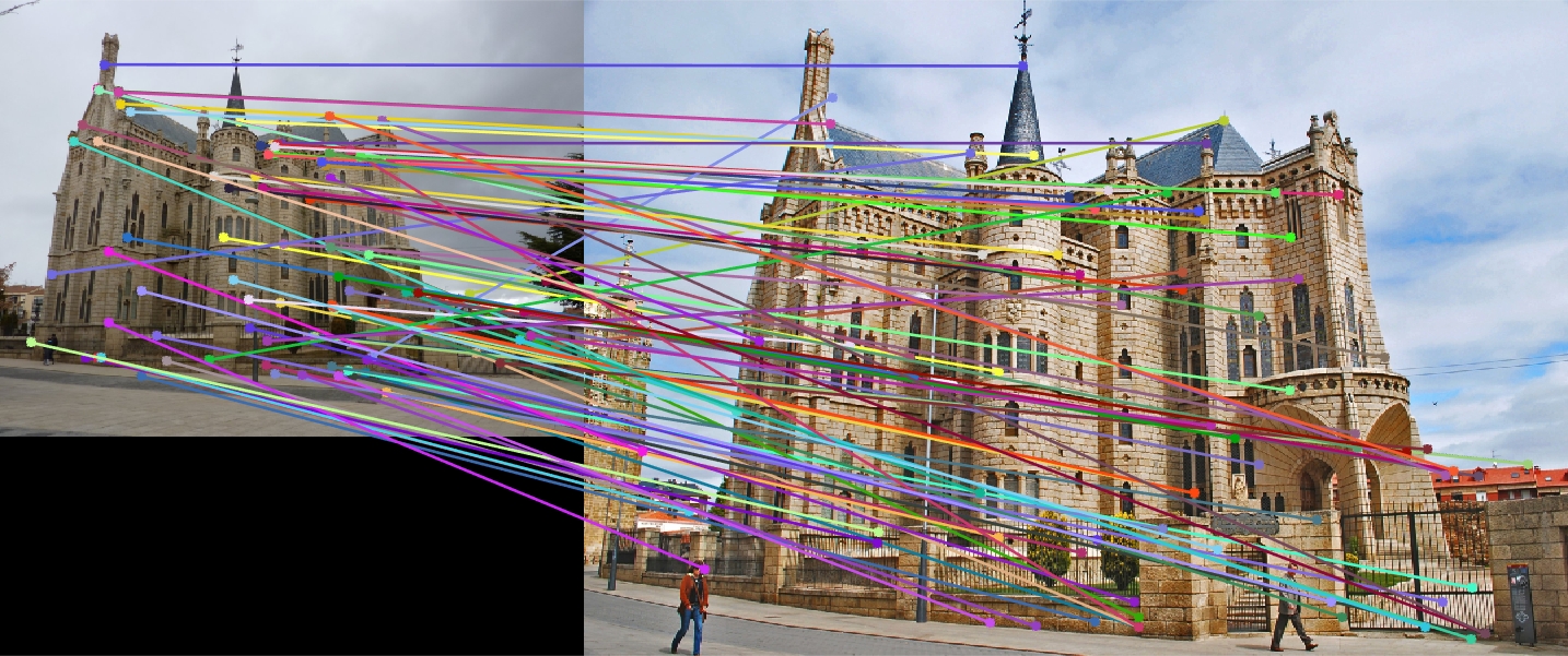
Finally, we show matches on extra image pairs. These results are obtained using Harris interest point detection with scaling, SIFT features with scaling, and NNDR matching.
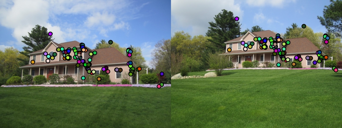
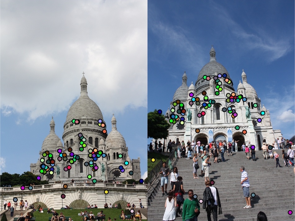
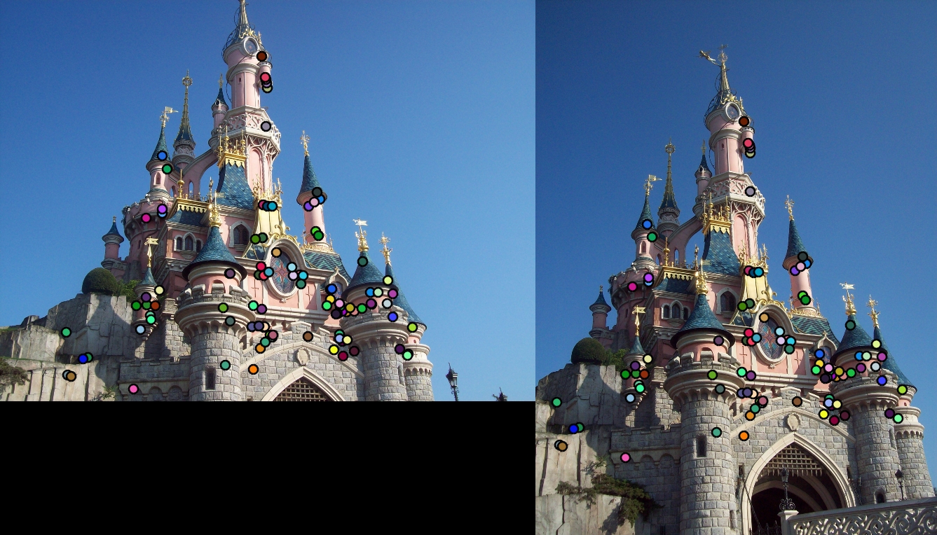
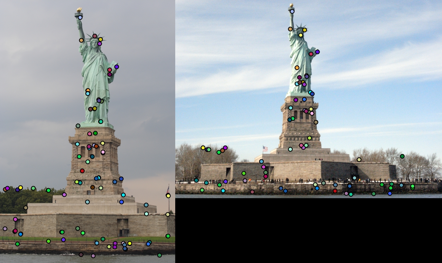
|