Project 2: Local Feature Matching
Attempt to feature match between similar images.
This purpose of the local feature matching project is to create an image matching pipeline that will match two similar images. These images might be taken from different perspectives and angles and we can see later on that these factors play a heavy role in the success rate. The image matching pipeline can be described as:
- Specifically, we start by identifying notable points in the image, which are called feature points.
- Then we create a feature descriptor for each feature point, which is a small matrix centered at the respective feature point.
- Finally, we will use a matching algorithm to identify the best matches given the descriptors.
Interest Points Retrieval
Specifically, I am using the harris corner feature detection algorithm. The purpose of an interest point is to find unique and uncommon points that could be used to indetify images, especially when you have a cluster of them. As suggested, this algorithm targets corners as the primary source of feature points, which is since creating a descriptor around it would change greatly if it were to move in any direction. If we had a edge, then it would be similar to another image if we moved an image along the edge direction, and a plane would be even more generic in that it would look like any other plane. In particular, I performed the following steps:
- I applied a 'small' gaussian filter onto the image via
imfilter - I calculated the horizontal and vertical derivatives of the filtered image by using
imgradientxyto create imageX and imageY - I calculated the outer products of imageX and imageY to yield imageXX, imageXY, and imageYY
- I then apply each of these above images with a 'larger' gaussian filter
- I use the above values to calculate the determinant and the trace of the matrix, and ultimately to find a scalar interest measure via
response = determinant - k*traceSquared; - Finally, I use non-max supression to get rid of noise around the corners to highlight a distinct feature point in that local vicinity.
%performing non-max supression

padding = feature_width/2;
local_maxes = colfilt(response, [padding padding], 'sliding', @max);
matched_filter = (response == local_maxes);
nonMaxSupression = response .* matched_filter;
colfilt on my computed response to perform a sliding window effect of size feature_width/2 x feature_width/2, and calculating the max value in each window. This function makes every value in that window to be the local maxima, which is why i need the following two steps. After that, I create a filter that retrieves all of the coordinates in which there was a local maxima, which i then apply onto my original image so that all of the local maximums are now only found at the correct coordinates.
Feature Point Descriptor Generation
I decided to use the 8 different orientations of a 3x3 sobel filter to represent the 8 gradient directions. I first applied a gaussian filter to smooth out the image, which helps reduce a lot of the noise in the image. I then applied each of the 8 filters onto the image.
gaussian_filter = fspecial('Gaussian', width , width);

for current_filter = 1:8
    sobel_filter = imfilter(image,filters(:,:,current_filter));
    all_filters(:,:,current_filter) = imfilter(sobel_filter,gaussian_filter);
end
After that, I calculated a descriptor for each interest point by cutting a 16 by 16 (or feature_width by feature_width) square with the interest point as the center. I then further divided it up into 16 equally sized cells, all of which are 4x4 (feature_width/4 by feature_width/4) and applied each of the 8 filters onto each cell. For each filter and cell combination, I would generate a single value to represent a gradient orientation for that specific combination by summing up all of the values in the cell, and store it in an entry in a 1 by 128 matrix, that would act like a histogram of gradient orientations for a given feature point descriptor. Finally, I would normalize the values and then store it into a larger matrix of k by 128, where k represents the number of feature points.
features = zeros(size(x,1), 128);
for feature = 1:size(x,1)
    feature_x = uint16(x(feature));
    feature_y = uint16(y(feature));
    current_feature = zeros(1,128);

    filter_index = 1;
    descriptor = all_filters(feature_y - width: feature_y + width  -1,
                             feature_x - width: feature_x + width  -1,
                             :); %feature_width x feature_width sized descriptor

    descriptor_cells = mat2cell(descriptor,
                                [cell_size,cell_size,cell_size,cell_size],
                                [cell_size,cell_size,cell_size,cell_size],
                                8); %4x4 cell array of smaller matrices

    for cellRow = 1:4
        for cellCol = 1:4
            filtered_cell = cell2mat(descriptor_cells(cellRow,cellCol));
            summed_cols = sum(filtered_cell, 1); %summing with respect to 1st dimension
            summed_plane = sum(summed_cols, 2); %summing with respect to 2nd dimension
            filtered_values = reshape(summed_plane,[1,8]); %reshaping a 1x1x8 matrix into a 1x8
            current_feature(:,filter_index:filter_index+7) = filtered_values; %inserting 8 numbers in at a time
            filter_index = filter_index + 8; %increment 8 because we add 8 values at a time
        end
    end

    current_feature = current_feature ./ norm(current_feature);
    features(feature,:) = current_feature;
end
Feature Matching
For this part of the code, I calculate the euclidean distance between every possible combination of feature points from the first image to the second image. After that, I sort the distances with respect to each point of the first image and retrieve the two smallest values. I then calculate the confidence between the two smallest points by dividing the second smallest point by the smallest point. I then append the indices of the feature in image1 with the appropriate match in image two in a k by 2 matrix. In addition to that, I include the corresponding confidence in k by 1 matrix as well. Finally, I take the top 100 confidences, and return that matrix as well as a matrix with the corresponding points to the top 100 interest points.
eucDistances = pdist2(features1, features2, 'euclidean');
[eucDistances, indices] = sort(eucDistances,2); %sort contents within each row (feature)
confidenceVector =(eucDistances(:,2) ./ eucDistances(:,1)); %calculating the ratio of the smallest two values of each row.

confidenceIndices = transpose(linspace(1,size(eucDistances,1),size(eucDistances,1))); %indices from 1 to the number of elements.
matches = [confidenceIndices, indices(confidenceIndices)]; %appending the indices from feature 1 to the appropriate index match in feature 2.

[confidences, ind] = sort(confidenceVector(confidenceIndices), 'descend');
confidences = confidences(1:100,:); %taking top 100 results
matches = matches(ind,:);
matches = matches(1:100,:);
Decision Table
| Decision | Accuracy |
|---|---|
| ----------------- get_interest_points.m Decisions ---------------- | ----- |
| small gaussian width = 4, large gaussian width = 8 | 78% |
| small gaussian width = 3, large gaussian width = 9 | 89% |
| alpha = 0.04 (Response Calculation) | 83% |
| alpha = 0.05 (Response Calculation) | 89% |
| alpha = 0.06 (Response Calculation) | 84% |
| ----------------- get_features.m Decisions ---------------- | ----- |
| smoothing image with Gaussian filter first | 89% |
| not smoothing image with Gaussian filter first | 66% |
| applying the sobel filter onto entire image | 89% |
| applying the sobel filter onto each descriptor | 72% |
Notable Algorithm Decisions
All of the above decisions are a comparison to the best set of variable values and decisions, which yielded an 89% match on Notre Dame.
One of the biggest contributors to the matching success has to be my decision to first apply a gaussian filter onto the image first before i generate my histograms for each interest point. This is largely due to the fact that the image has a lot of noise, and thus has a larger liability to create inaccurate descriptors than with the gaussian blur. As noted above, the accuracy spiked tremendously from 66% match to an 89% match.
Another key decision was to apply the sobel filters first onto the entire image before generating any descriptors. The reasoning was because of boundary effects that impacted the descriptor generation and overall results. By applying the sobel filters onto the entire image, we can hide the boundary effects better since a majority of the interest points will be towards the center of the image. This not only caused a spike from 72% to 89%, but it ran much faster as well due to the fact that it doesn't need to call imfilter 8 times for each interest point.
Another one of the big decisions that i made was that I decided to apply all 8 of the sobel filters onto my image at once and created a w by h by 8 matrix where w and h are the width and height of the image being passed in, so that there are 8 different filter applied versions in one 3D matrix. I then would iterate over all of the interest points and cut out a submatrix out of size feature_width by feature_width and it centering at the feature point so that there is a 16 by 16 by 8 matrix currenty. Then I divide it into 16 equal sized cells of 8 layers to create sixteen 4 by 4 by 8 matrices. For each one, I sum up the values in the corresponding cell such that there is a single value to represent each cell with a different applied filter. This yields a 1 by 8 matrix of values that correspond to each gradient applied cell that I would insert into the 1 by 128 matrix. I did it this way because it overall is faster than how I had originally approached it where I had 4 for loops, but since I am calculating 8 values at a time, it eliminates the need for a another forloop where i apply each filter onto each descriptor. This was a tremendous speed up from about 5 minutes on notre dame to about 20 seconds.
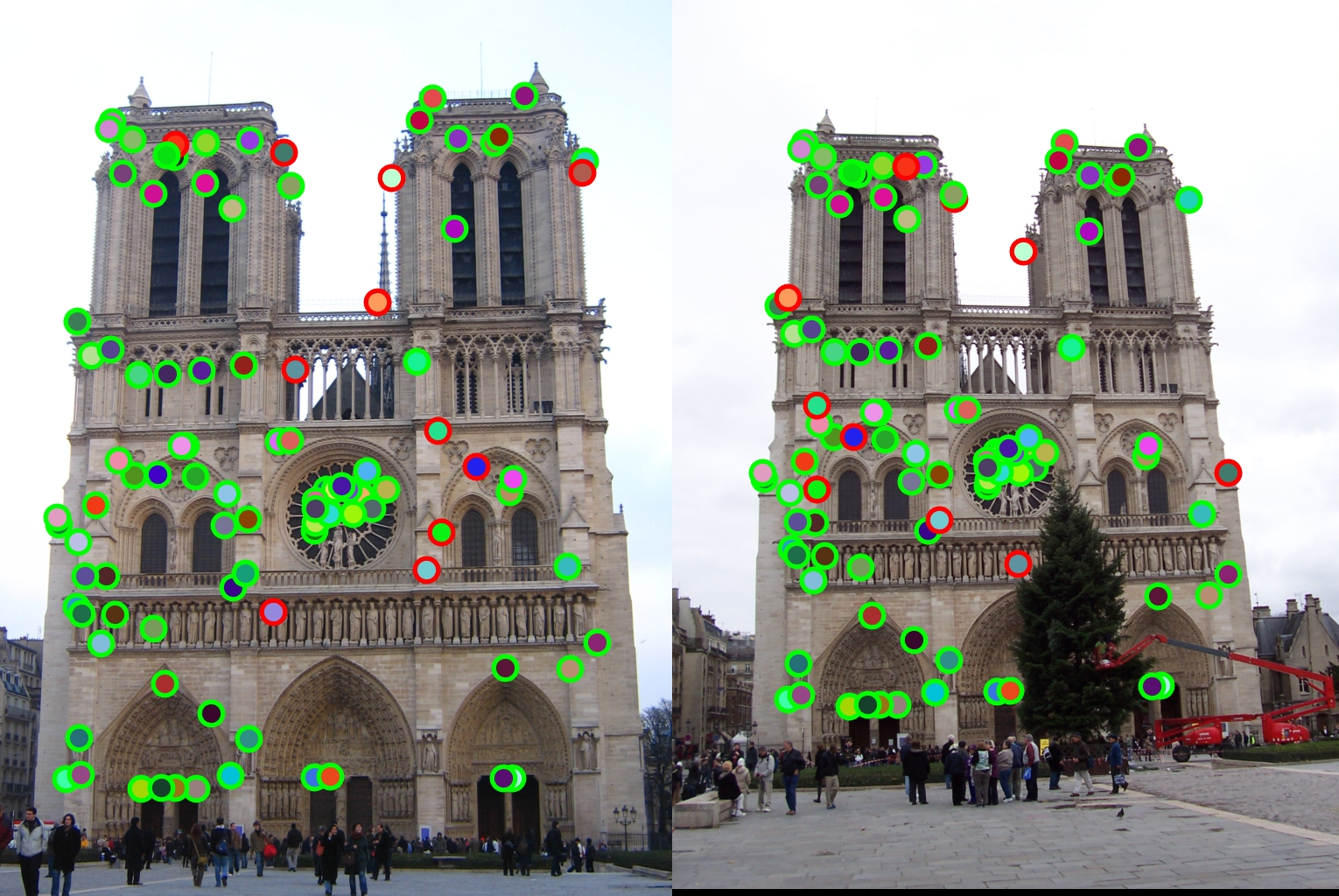
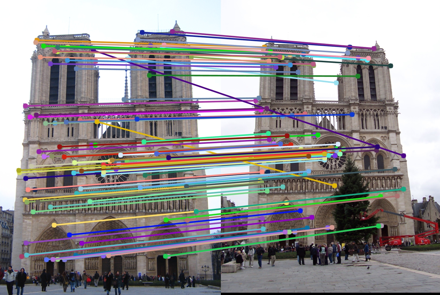
Notre Dame - 89% Match
Overall the described algorithm above was fairly successful in terms of matching the two images together. After finetuning all of the variables, I was able to get a max of 89%. Since I took the top 100 points, this meant that 11 of them were matched incorrectly. Of those 11, a majority of them had understandable reasons as to why they were wrong, such as having the same type of pillar in the background as it's corresponding match, but just in a different location. Because of the fact that there were a lot of the same patterns throughout the entire architecture of the building, there was some confusion as to which of the many structures it might be related to, thus the lower accuracy compared to Mt. Rushmore.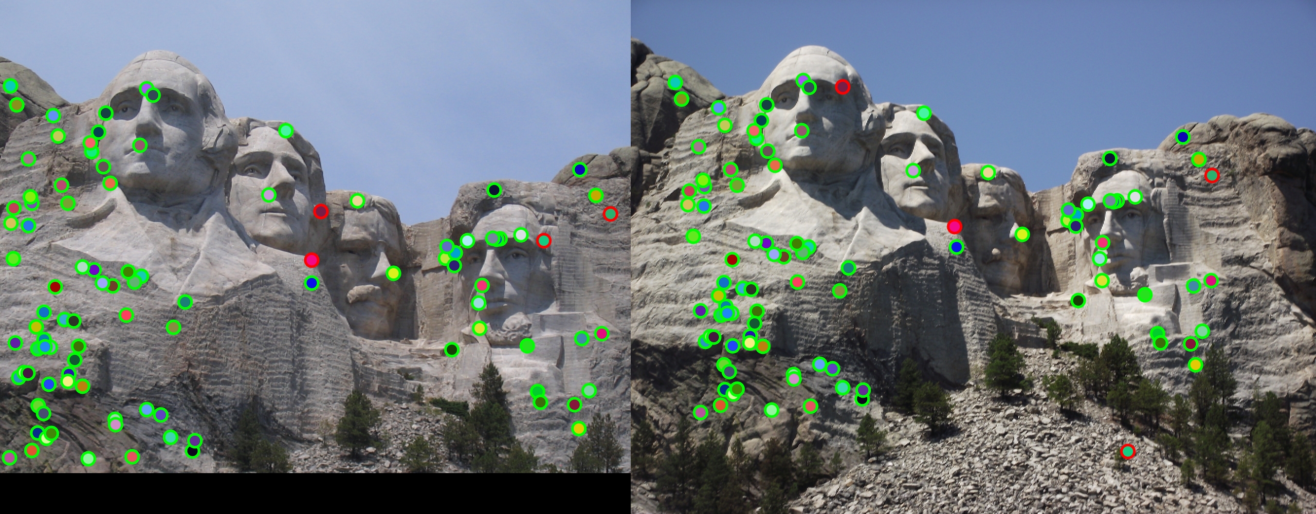
Mount Rushmore - 96% Match
As noted before in the Notre Dame analysis, Mt. Rushmore performed spectacularly under the given feature matching pipeline. It received a 96% match, meaning only 4 of which were mistakened for. My reasoning as to why this performed so well is because this landmark or image had a lot less repeating patterns, meaning there were higher confidence values, and less of a chance to get a mismatch with a similar patterned background.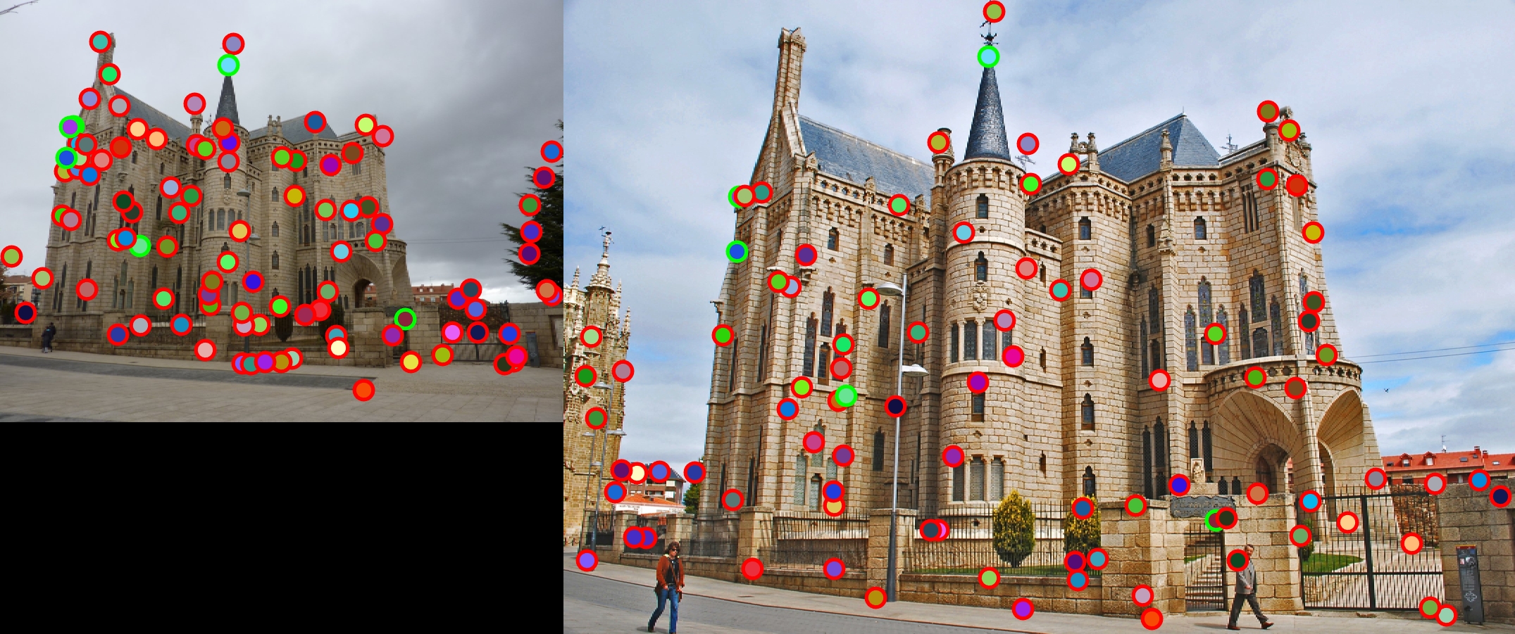
Episcopal Gaud - 4% Match
This image by far performed the worst. It received a 4% match, which could be due to many factors such as scale and very similar patterns across the entire architecture of the building.