Project 2: Local Feature Matching
This project report focuses on the implementation of a SIFT-like pipeline for doing instance level feature detection and matching.
Interest point detection
The first part of the pipeline is interest point detect, i.e. finding features in the image that is likely to be identified in other images of the same phyiscal location.
I chose to implement a basic version of the Harris corner detector. First I compute the image gradients, then the second moment matrix and the Harris score for each pixel in the image.
	% output is the Harris corner image
	output = (Sxx .* Syy) - (Sxy .^ 2) - ALPHA * ((Sxx + Syy) .^2);
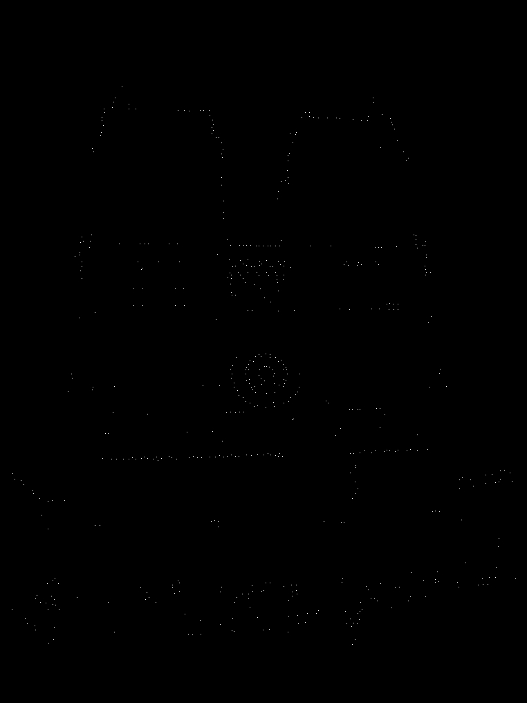
Visualization of the Harris corner response matrix.
The corner responses are then filtered so that any responses below the threshold HAR_THRESHOLD is suppressed. That is because they are presumed to be egdes or flat surface. All interest points near the egde of image are also suppressed since a patch around them cannot be extracted in the feature descriptor step. Finally all non-maxima points are suppressed using a sliding window. This is done to speed up the pipeline by giving fewer and distinct interest points. Essentially the non-maxima suppress selects the best point in a point cluster around a good feature in the image rather than all of them. This also reduces any potiential confusion when matching since there are fewer similar looking points.
Parameters and efficiency
Visual inspection of the Harris corner response matrix seems to indicate good performance. The points found are in the corners of the Notre Dame. Using non-maxima suppression speeds it up signifacantly and increases accuracy by about 3 procent points.
- GAUSS_SIGMA - The standard deviation of the Gassian used to compute the second moment. Larger means that the surrounding gradients affects have a greater influence on the Harris score. I found that 1.9 was optimal.
- GAUSS_WINDOW - The size of the window used then filtering with the Gaussian. Larger means that the Harris score was sampled from a larger area. I used the 16 px (the feature_width). It makes sense that the Harris score should be calculated upon the same area as the feature descriptor.
- ALPHA - Used to compute the Harris score. According to Szeliski 0.06 is in general considered optimal and testing proved this correct.
- HAR_THRESHOLD - The threshold for the Harris score. Larger means fewer interest points but also less point to match. 0.07 was experimentally found to be optimal.
- NON_MAX_WINDOW - The window size of the non-maxima suppression. Larger means fewer interest points and also sparser features. I found that a 3x3 strikes a balance between performance and accuracy.
Feature descriptors
From the interest points the pipeline creates SIFT-like feature vectors for each interest point. These 128 dimensional vectors acts like fingerprints that are unique to features in the image. Ideally they are also robust to scaling and lighting changes.
The features are created by looking at 16x16 pixel patches around the interest point. Then calculating the magnitude and direction if the image gradients in the patch. After that a gaussian filter is applied to the magnitudes to make the descritor less sensitive shifts in the images.
The patch is then divided into 4x4 cells that are processed one by one. For each cell an eight bin gradient magnitude histogram is computed. These 4x4x8 bins will serve as out 128 dimensions feature vector. To make the feature vector further resistant to small shifts trilinear interpolation amongst the bins are used to propagate the bins values to nearby bins in the patch. This last step increased accuracy by about five percentage points.
To make the feature vectors more uniform they are normalized, clamped to 0.2 and the renormalized. Clamping and normalizing improved the accuracy by 5 percentage points.
Parameters and efficiency
The SIFT-like feature descriptors are superior to the raw pixel intensity template methods since they are more resistant to changes in lighting, scaling and rotation.
- GAUSS_SIGMA - This variable determines how big standard deviation to use when filtering the gradient magnitudes in the patch. Higher means that neighbouring gradient have greater impact. This variable had a great influence on the accuracy, around 20 percentage points. Experimentally 1.8 was found to be optimal.
- TRI_DAMP - When performing trilinear interpolation how much to dampen the magnitude before adding to nearby bins. Lower means less influence. 0.8 was found to give maximum accuracy boost. Too much or too little made the interpolation either ineffective or destructive to the unique features of each cell.
Feature matching
For each feature in the second image I found the two closest points in the feature space (using the euclidean distance). I then calculated the Nearest Neighbour Distance Ratio Test, i.e. matches with a ratio better than NNDR_THRESHOLD were considered good. The result was sorted from best ratio to worst. A small ratio means that the nearest neighbour is much more similar than the next nearest, thus implying that the match is good relative to all other possible matches.
[D, I] = pdist2(features1, features2,'euclidean','Smallest', 2);
for i = 1:size(features1, 1)
   d1 = D(1, i);
   d2 = D(2, i);
   nndr = d1/d2;
   if nndr <= NNDR_THRESHOLD
        matches = [matches; [I(1,i) i]];
        confidences = [confidences, nndr];
   end
end
Parameters and efficiency
- NNDR_THRESHOLD - In Distinctive Image Features from Scale-Invariant Keypoints from 2004 Lowe asserts that 0.8 is a good ratio that filters out 90% of false positives, while discarding less than 5% correct matches.
Discussion
This project is very open to improvements both in the pipeline itself and through tweaking of the parameters. I settled on implementing a SIFT-like pipeline and tweaking the parameters as best I could.Final accuracy
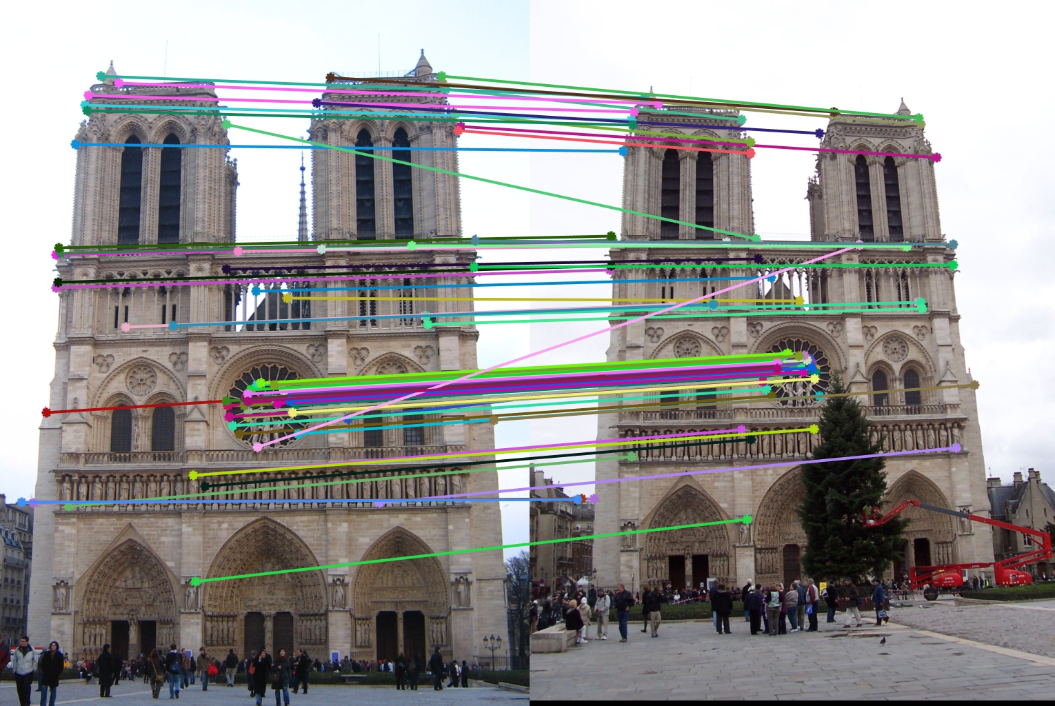
The table below shows my algorithms accuracy on the different images.| Accuracy (at NNDR=0.8) | Accuracy (100 best) | Matching image (100 best) |
| 84% (out of 76) | 77% |
|
| 38% (out of 16) | 22% |
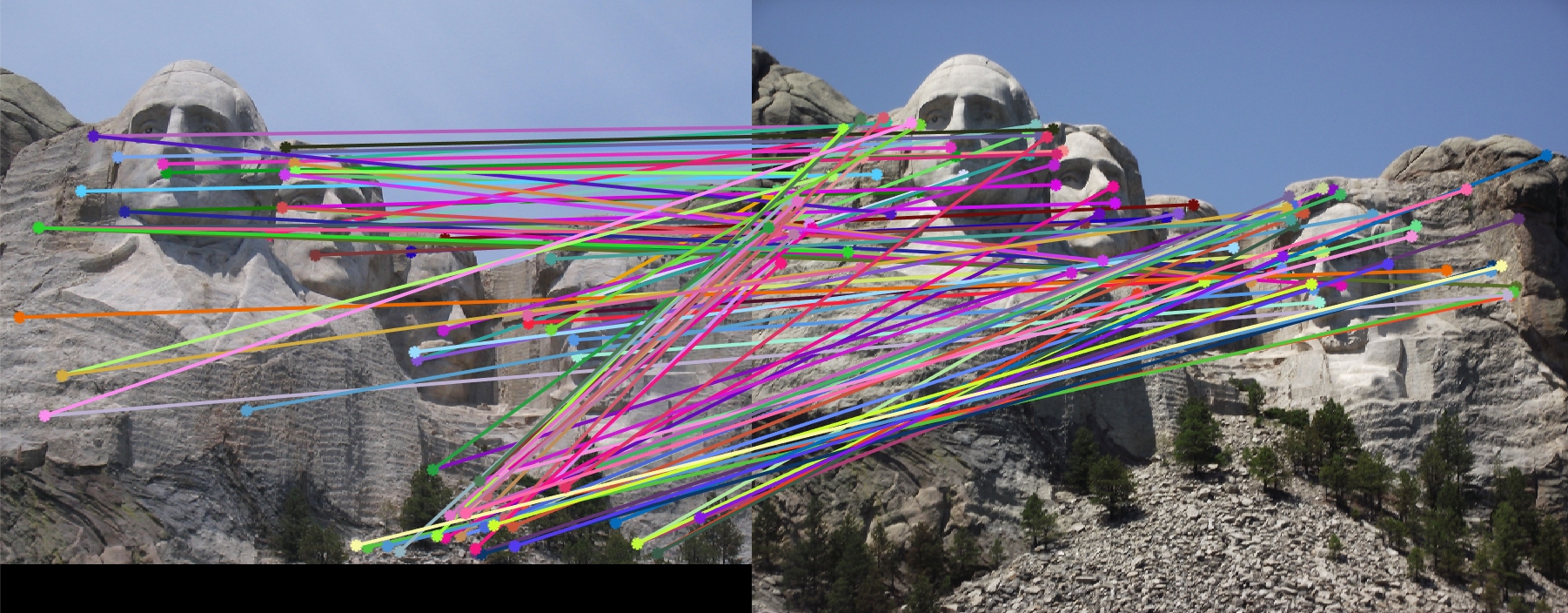
|
| 11% (out of 11) | 6% |
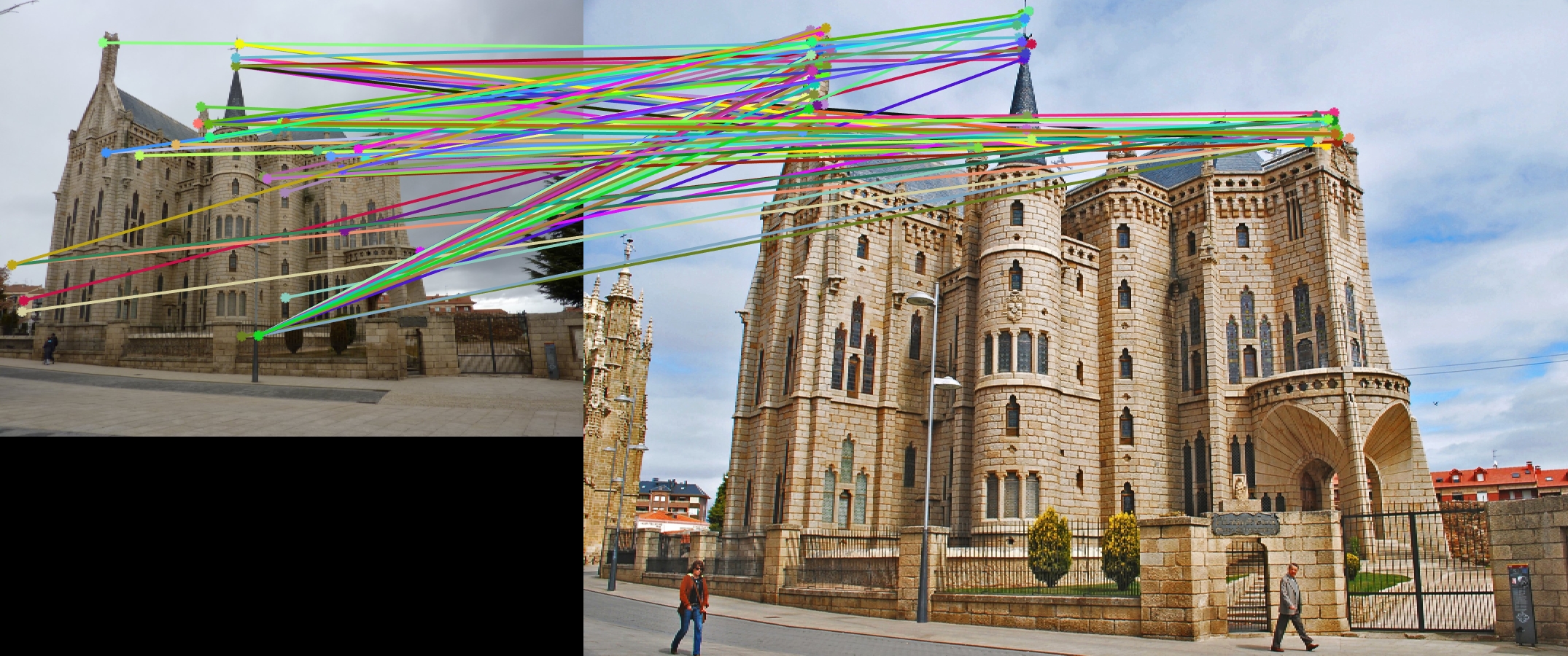
|