Project 2: Local Feature Matching
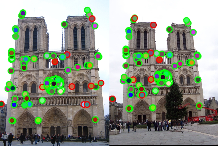
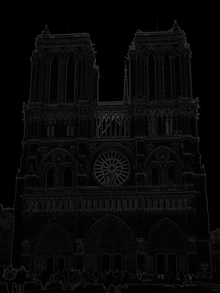
Keypoint detection accuracy is 139/149 (93.29%) for 'Notre Dame'.
In this project, the goal is to create a local feature matching algorithm using techniques described in Szeliski chapter 4.1. Local feature matching basically includes three major steps.
- Interest Point Detection: A Harris corner detector is implemented as interest point or keypoint detector.
- Local Feature Description: A simplified version of the famous SIFT pipeline is implemented for feature description.
- Feature Matching: An Euclidian distance based nearest neighbor approach is followed for feature matching. Also, instead of simple thresholding, ratio testing is used to get more accurate results.
Details of above steps are described in the following with explanatory figures and test results. The overall accuracy of the proposed feature matching algorithm is 139/149 (93.29%) for 'Notre Dame' image pairs.
1. Interest Point Detection
In this step, get_interest_points() function is implemented. Interest points are detected by applying Harris corner detection method. Further noise elimination steps such as Hysteresis Thresholding and Non-Maxima Suppression are applied to detected corner candidates. In what follows, the details and the implementation of these sub-steps are presented.
1.0. Prepare the input parameters for the functions below.
% 0. Prepare parameters. Each parameters have comments for possible values could be tuned.
if nargin < 3
    filter_size=3;% 3, 5, 7
    alpha = .04;% .04, .05, .06
    lower_th=.1;% .05, .1, .15, .2
    higher_th=.8;% .6, .7, .8, .9
    radius=2;% 1, 2, 3
end
% 1. Compute the x and y derivatives of the image. Sobel gradient operator is choosen for better result.
[Ix,Iy]=imgradientxy(image,'sobel');
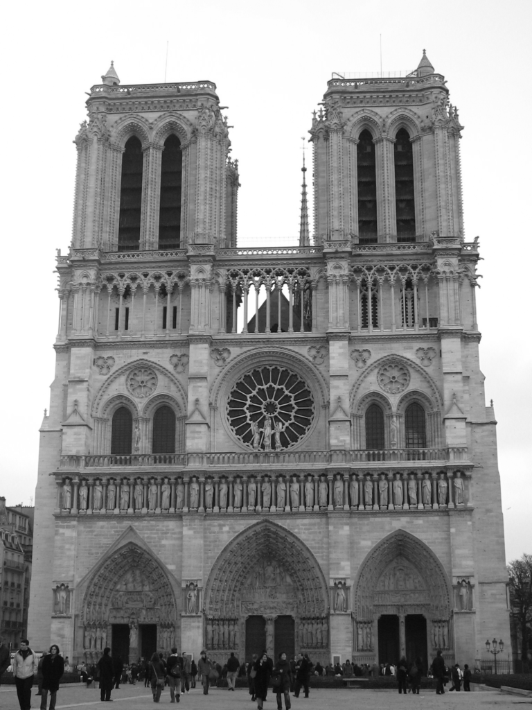
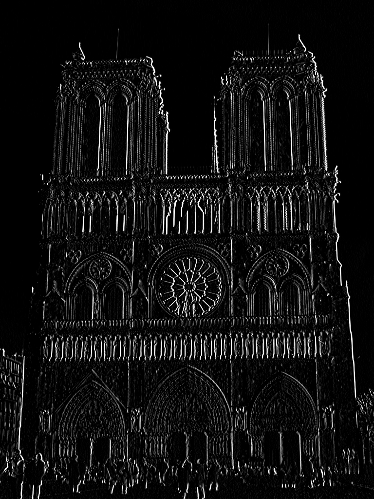
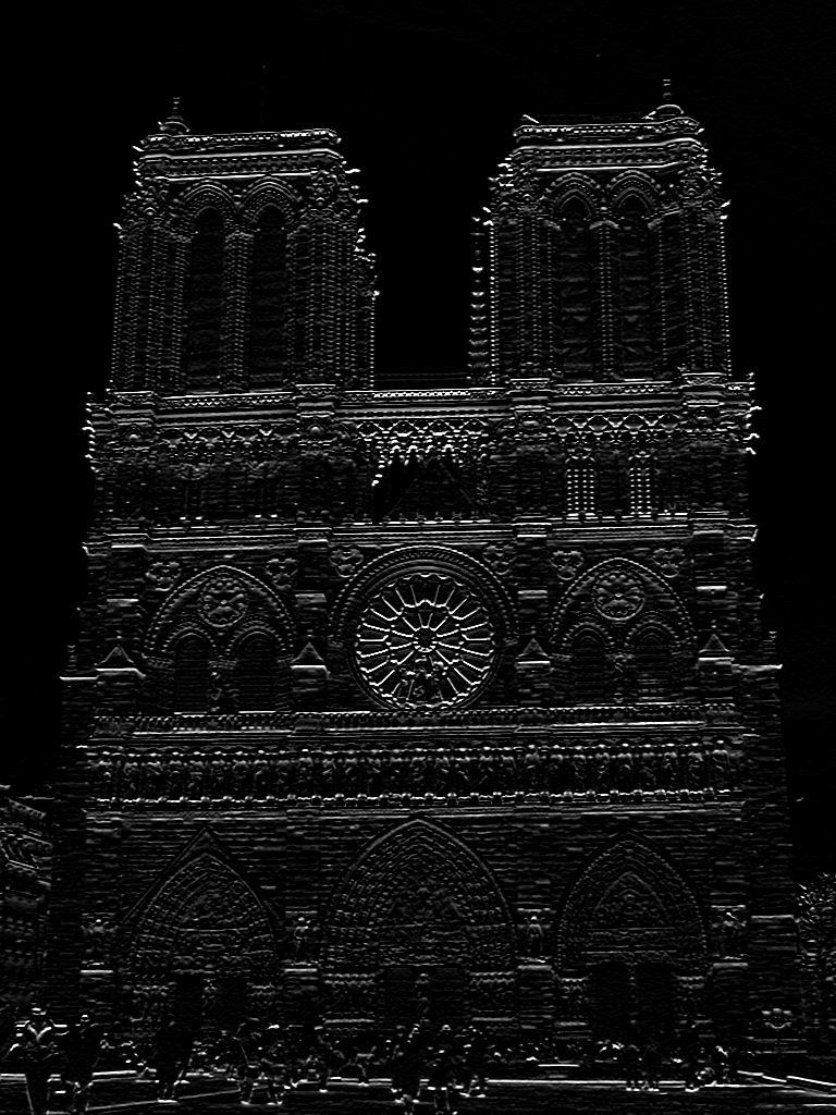
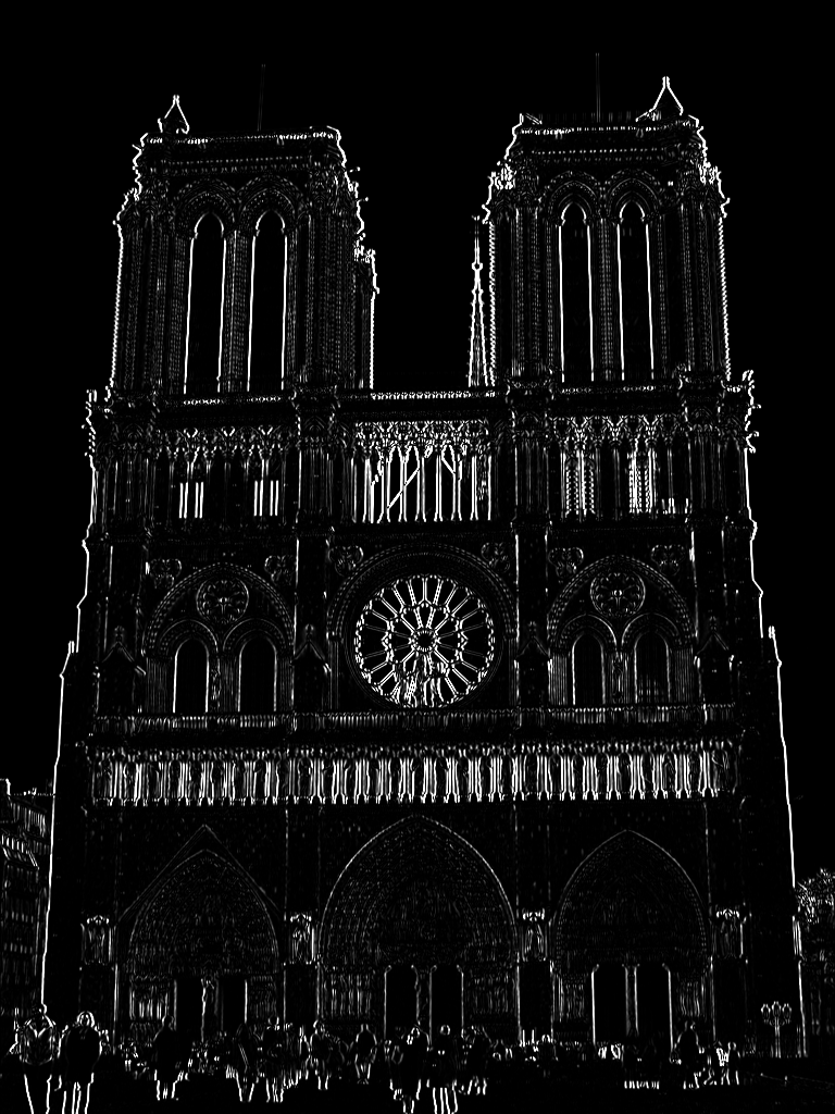
Left to right, original grayscale image and its x and y derivatives (Ix and Iy).
% 2. Compute products of derivatives at every pixels
Ix2=Ix.^2;
Iy2=Iy.^2;
Ixy=Ix.*Iy;
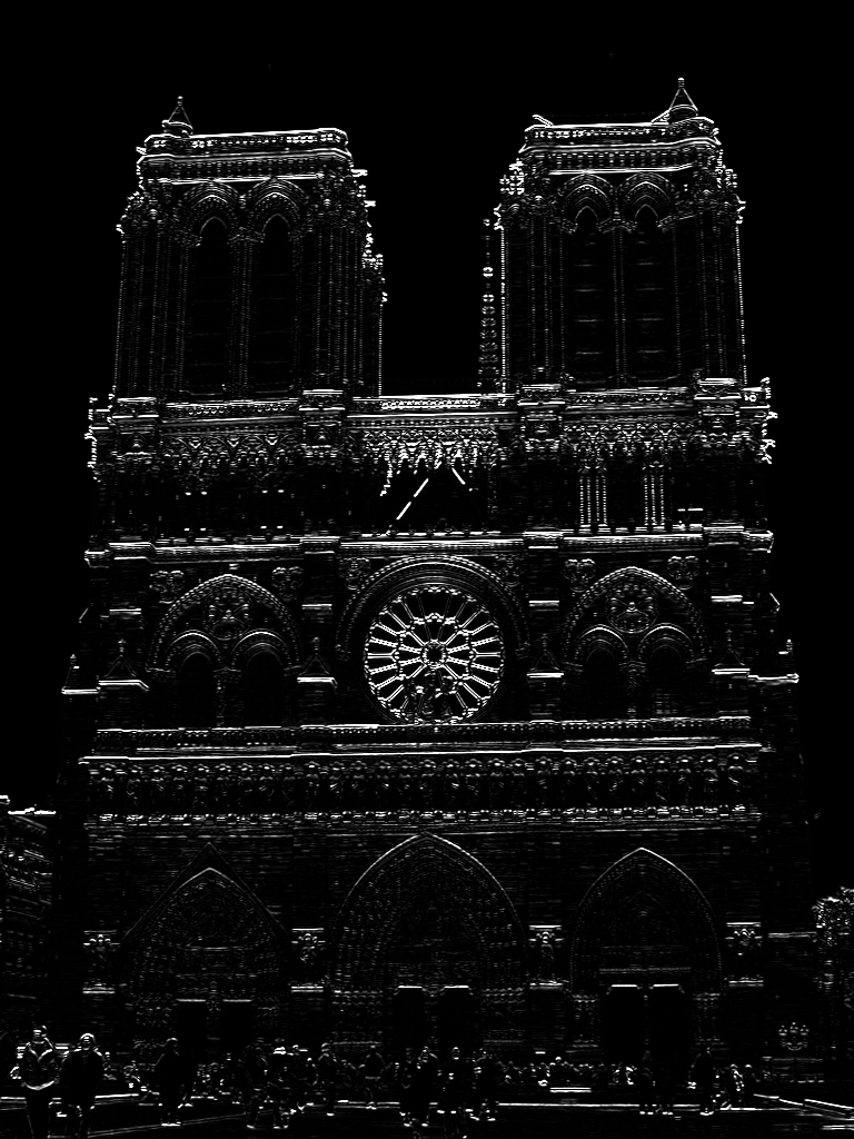
Left to right, squares of x and y derivatives (Ix2 and Iy2) and products of Ix and Iy (Ixy).
% 3. Apply Gaussian filter
h=fspecial('gaussian',filter_size,filter_size);
Ix2=imfilter(Ix2,h);
Iy2=imfilter(Iy2,h);
Ixy=imfilter(Ixy,h);
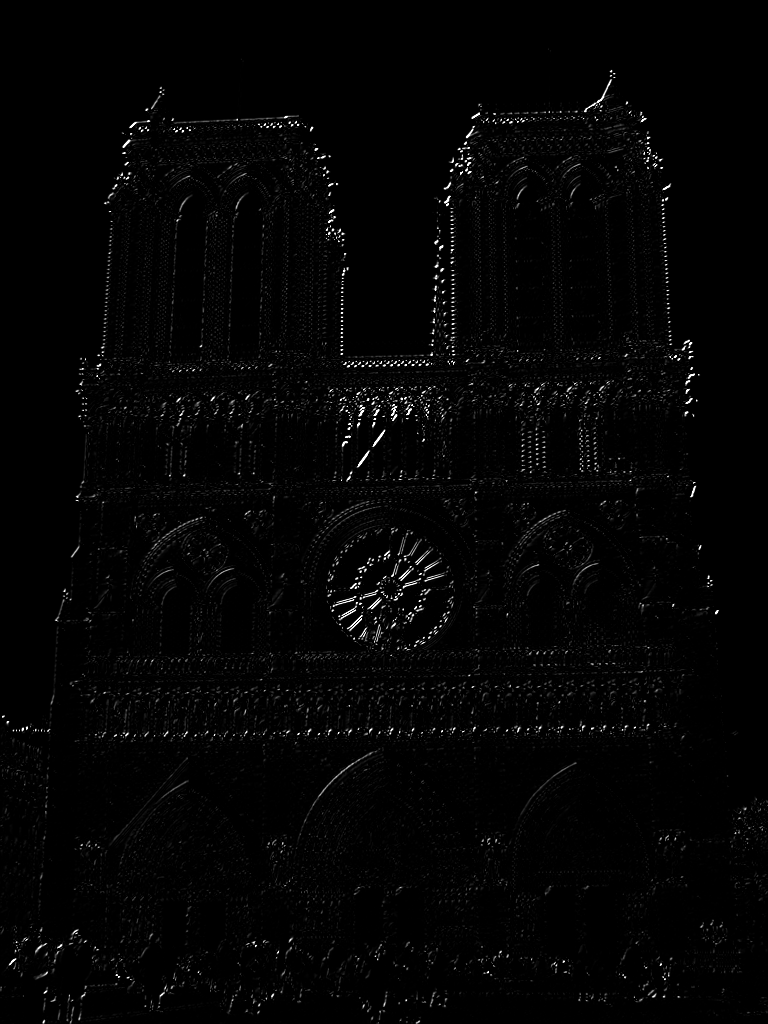
Left to right, Gaussian filtered derivatives Ix2, Iy2, Ixy.
% 4. Compute the response of the detector at each pixel
R= (Ix2 .* Iy2) - (Ixy.^2) - alpha*(( Ix2 + Iy2 ).^ 2);
% 5. Apply Hysteresis thresholding
C=(lower_th<R) & (R<higher_th);
R(~C)=0;
% 6. Apply Non-Maxima Suppression
% 6.1 Extract local maxima by performing dilation with disk shape in 'radius'
mx = imdilate(R, strel('disk',radius));
% 6.2 Create bordermask to exclude points within radius of the image boundary.
bordermask = zeros(size(R));
bordermask(radius+1:end-radius, radius+1:end-radius) = 1;
% 6.3 Find points in the corner strength image that match the dilated image
% and also apply bordermask and hysterisis threshold again.
Rmx = (R==mx) & C & bordermask;
% 6.4 Find row,col coordinates.
[y,x] = find(Rmx);
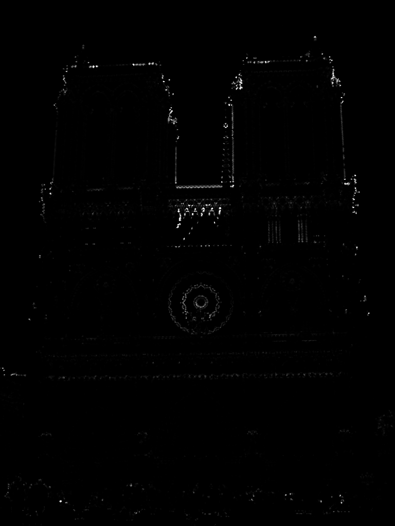
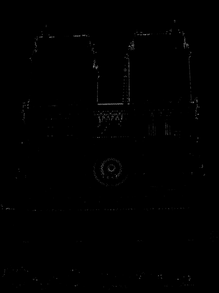
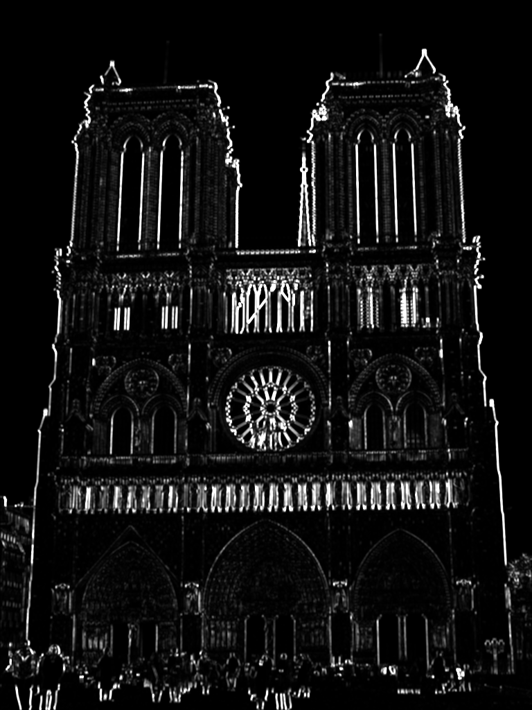
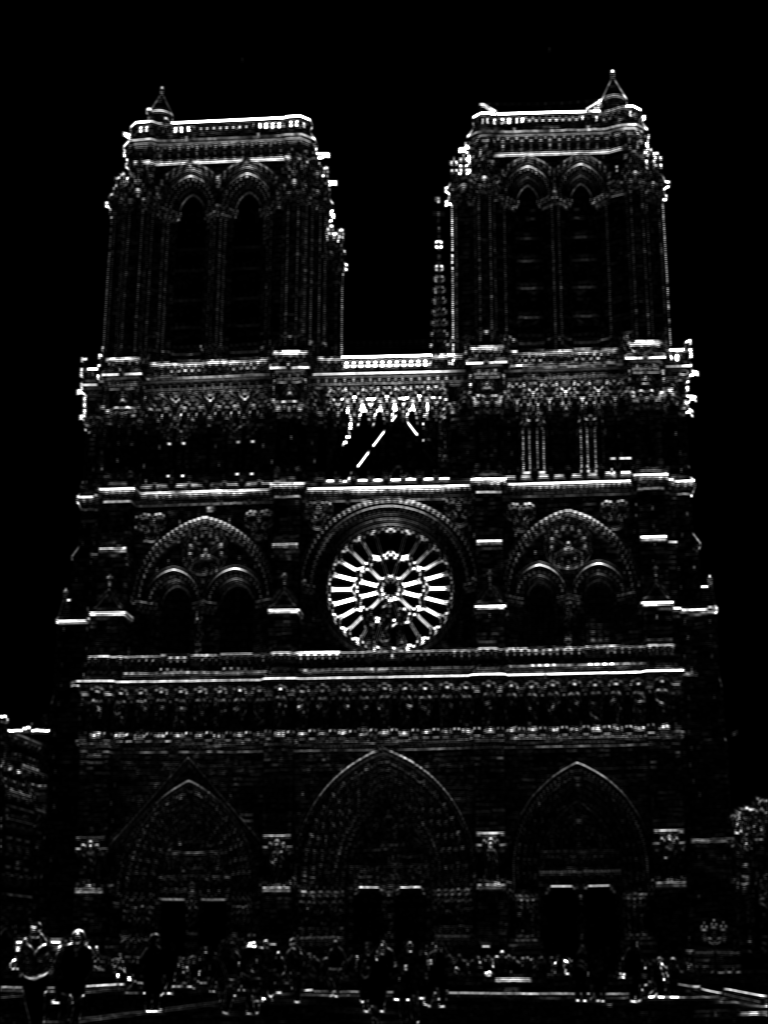
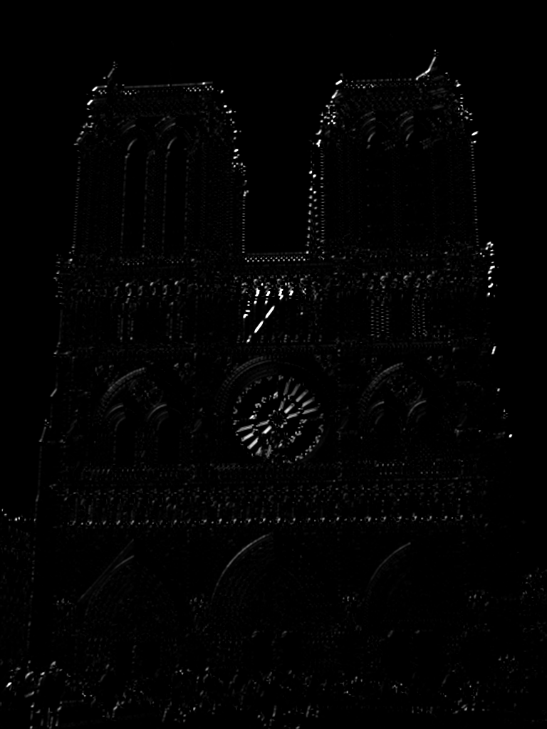
Left to right, Harris response image, Hysteresis thresholded image and Non-Maxima suppression applied image from steps 1.4, 1.5 and 1.6, respectively.
2. Local Feature Description
In this step, a SIFT like feature descriptor calculation is implemented. For simplicity, the descriptor is not scale or orientation invarient. Here is the sub-steps of get_features() function. To keep the code's completeness, the steps are enumerated below with corresponding figures.
- First, the directional gradients and calculated, then, the magnitude and orientation of each gradients in image is measured. Orientation is changin from -180 to 180 degrees. Here is the magnitude and orientation of given image above (left to right, magnitude and orientation).
- Iterate around each keypoints calculated in first step above.
- Exclude the border region of the image to escape from exceptions.
- Pick the region around each keypoint to calculate feature vector. In this setting, the region is 16x16 dimension.
- Divide each 16x16 regions around each keypoints into 16 cells with 4x4 dimension.
- Iterate for each orientation changing 45 degrees at each time. Get the magnitude sum for corresponding orientation region. This yields 8 histogram bins for each cell. At the end, 16x16 region yields 4x4x8=128 feature values.
- Normalize the 128-dim vector to 1 and apply thresholding to gradient magnitudes to avoid excessive influence of high gradients. Then, renormalize.
% 0. Invert x and y indices for clarification. And prepare parameters.
x1=ceil(y);
y=ceil(x);
x=x1;

cd=feature_width/4; % Cell width and height. Feature dimension 'fd' parameter.
fd=cd*cd*8; % Feature dimension. 8 is the bin count representing 8 orientation.
features = zeros(size(x,1), fd); % Create returning feature matrix.


% 1. Calculate the directional gradients by using 'central' method.
% Central difference gradient: dI/dx = (I(x+1)- I(x-1))/2
% Central method is choosed since it gives best result among all.
[Gx, Gy] = imgradientxy(image,'central');
% Calculate the magnitude (mag) and orientation (pha- [-180,180]) of each gradients.
[mag, pha] = imgradient(Gx, Gy);

% 2. Iterate on each key points
for k=1:numel(x)
    % 3. Escape from borders.
    hf=feature_width/2; % half size of the feature width. In this case 8.
    if (x(k)<=hf)||(y(k)<=hf)||(x(k)>=size(mag,1)-hf+1)||(y(k)>=size(mag,2)-hf+1)
        continue;
    end

    % 4. Create 16 x 16 (feature_width x feature_width) region around the keypoint.
    mag_reg=mag( x(k)-hf+1:x(k)+hf , y(k)-hf+1:y(k)+hf );
    pha_reg=pha( x(k)-hf+1:x(k)+hf , y(k)-hf+1:y(k)+hf );

    descriptor=zeros(1,fd); % Descriptor vector keeping feature vector.
    descI=1;

    % 5. Divide 16x16 regions into 16 4x4 cells. And, iterate on each.
    for i=1:cd
        for j=1:cd
            % Get (i,j)th cell.
            mag_sub=mag_reg( (i-1)*4+1:i*4 , (j-1)*4+1:j*4 );
            pha_sub=pha_reg( (i-1)*4+1:i*4 , (j-1)*4+1:j*4 );

            % Keeps sum of magnitudes for each orientation
            mag_sums=zeros(1,8);

            % 6. Iterate on each cell and get gradients on 8 direction.
            % Directions change 45 degrees each time.
            for angle=0:45:359
                c1=-180+angle;
                c2=c1+45;
                mag_sums((angle/45)+1)=sum(mag_sub(pha_sub>c1 & pha_sub<=c2));
            end
            descriptor(1,descI:descI+7)=mag_sums;
            descI=descI+8;
        end
    end

    % 7. 128-dim vector normalized to 1. Then, threshold gradient
    % magnitudes to avoid excessive influence of high gradients.
    % This step is repeated for a couple of time to increase accuracy.
    descriptor=normr(descriptor); % Normalize to 1.
    descriptor( abs(descriptor)>0.2 )=0.2;% clamp gradients>0.2
    descriptor=normr(descriptor); % Renormalize
    descriptor( abs(descriptor)>0.2 )=0.2;
    descriptor=normr(descriptor);
    descriptor( abs(descriptor)>0.2 )=0.2;
    descriptor=normr(descriptor);


    features(k,:)=descriptor;
end