Computer Vision Project

Project 2: Local Feature Matching

In this project, our main goal is to be able to identify and match points between two images of the same object or place of interest. This is broken down into roughly 3 steps:

Find key interest points
Create features for all interest points
Match interest points between images

We will be walking through the development of the pipeline and highlight the various methods and tweaks that improved performance. For this project, our performance will be focusing on the accuracy of our top 100 matches between two images. These top 100 matches are the most confident matches that we find between the two images.

The Images

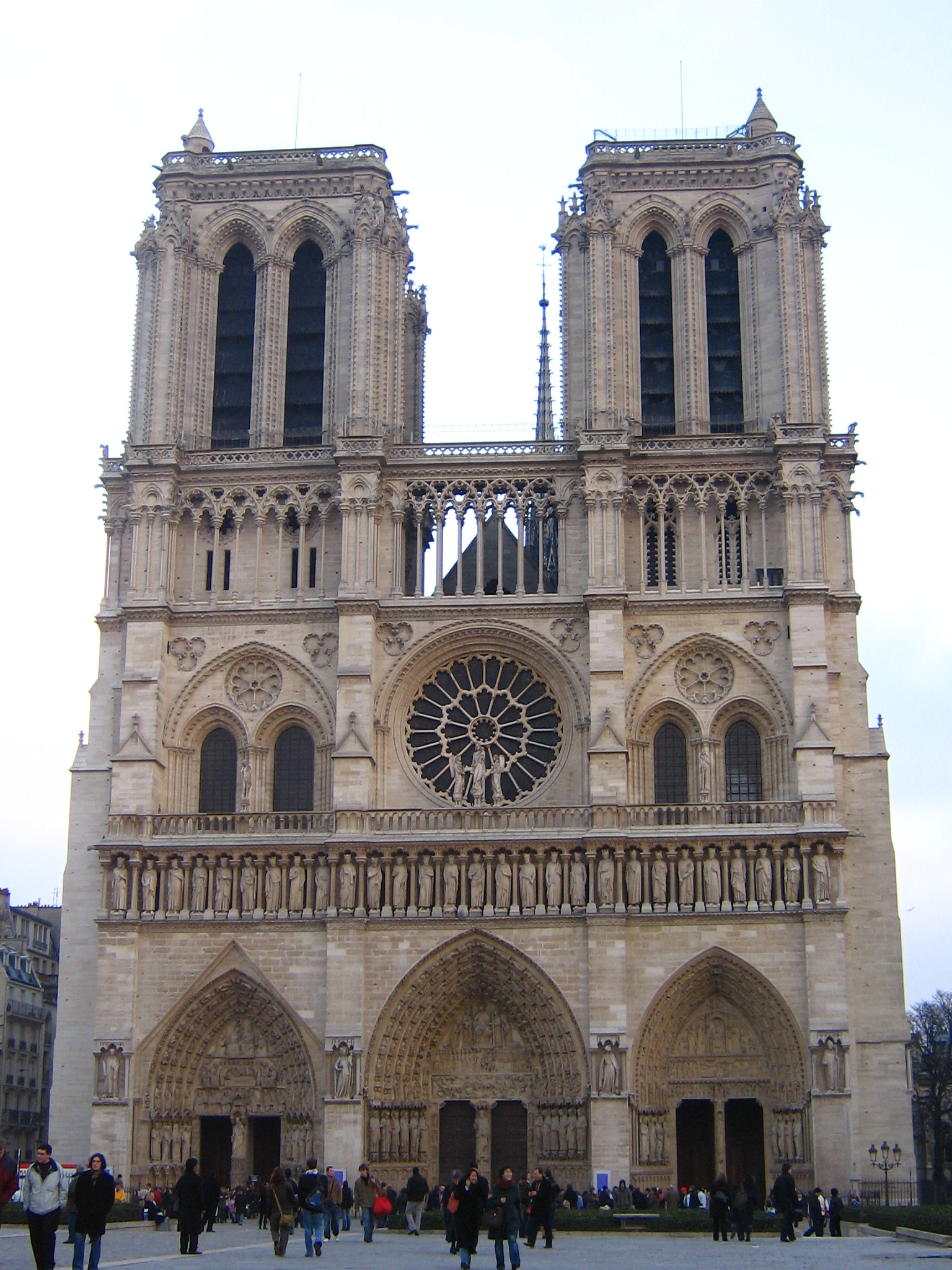
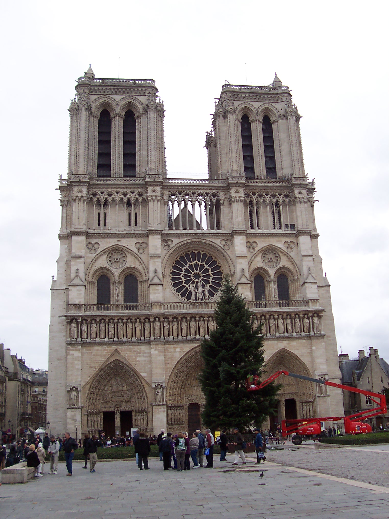
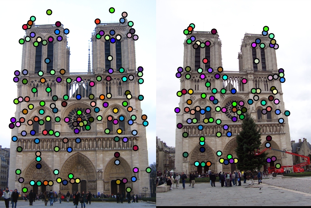
Notre Dame

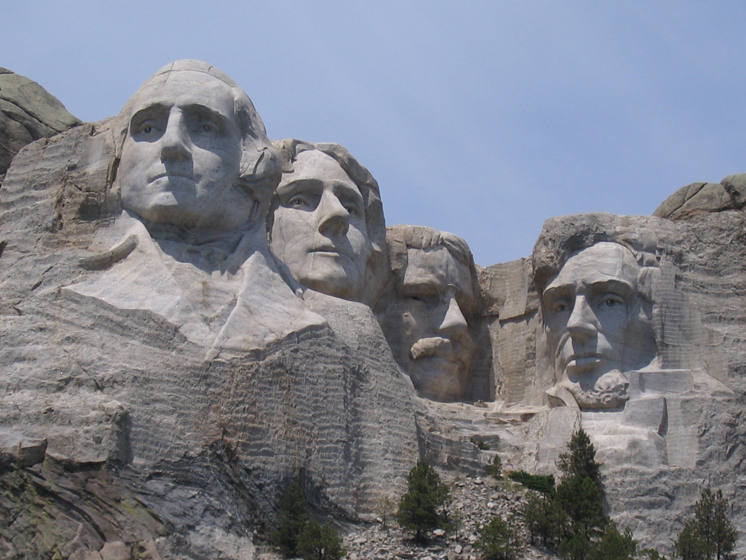
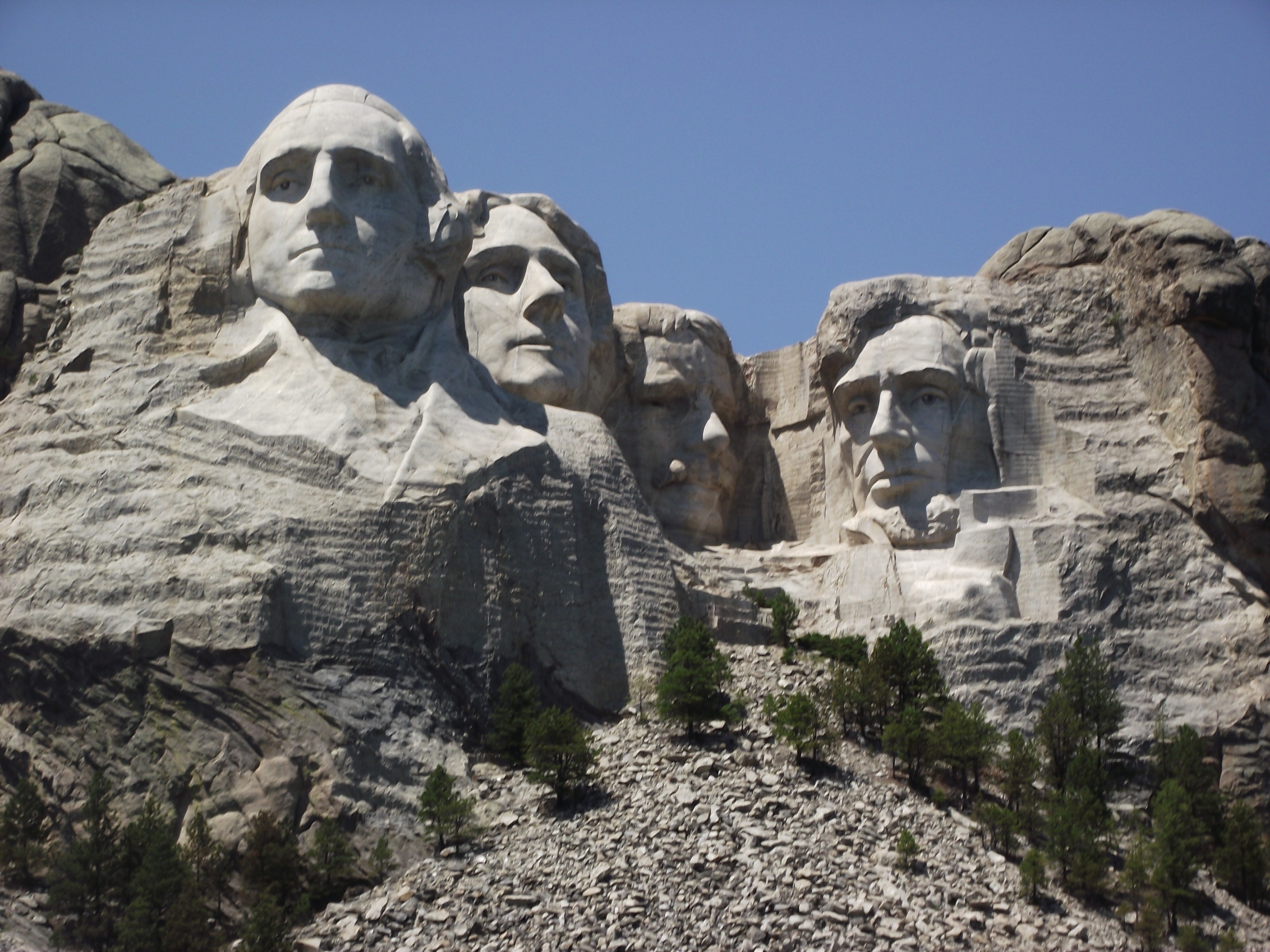
Mount Rushmore

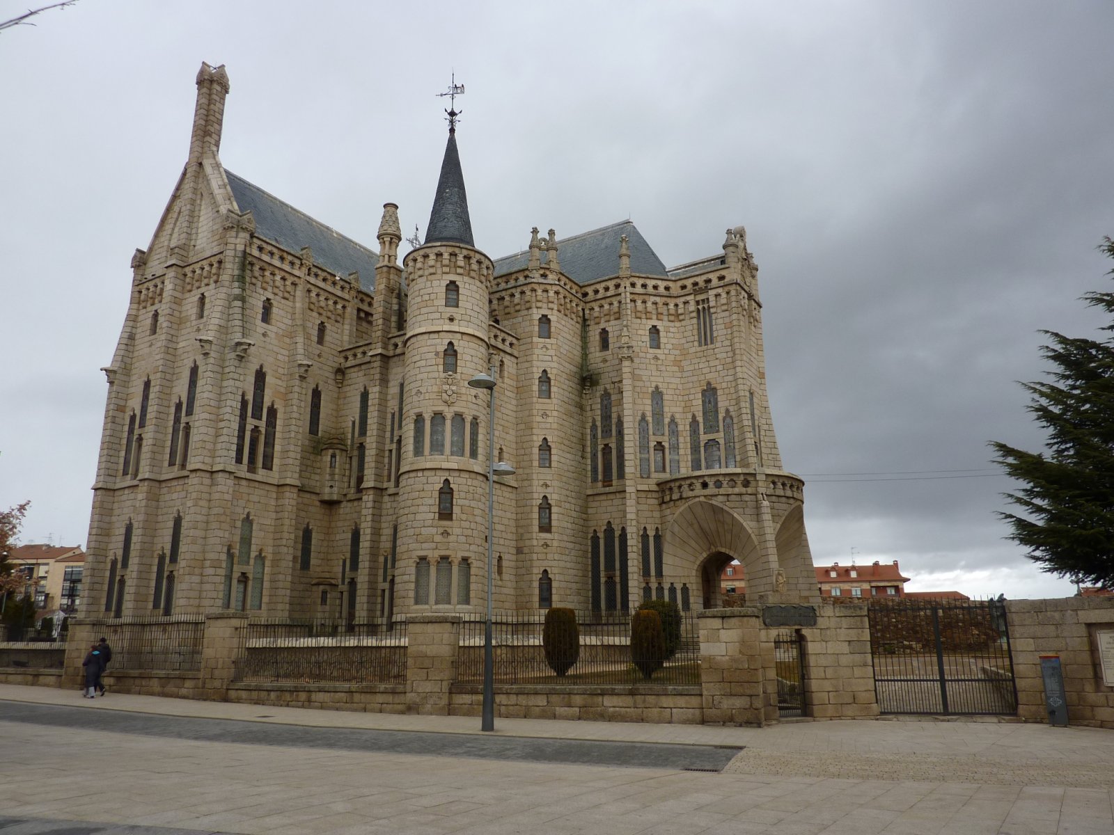
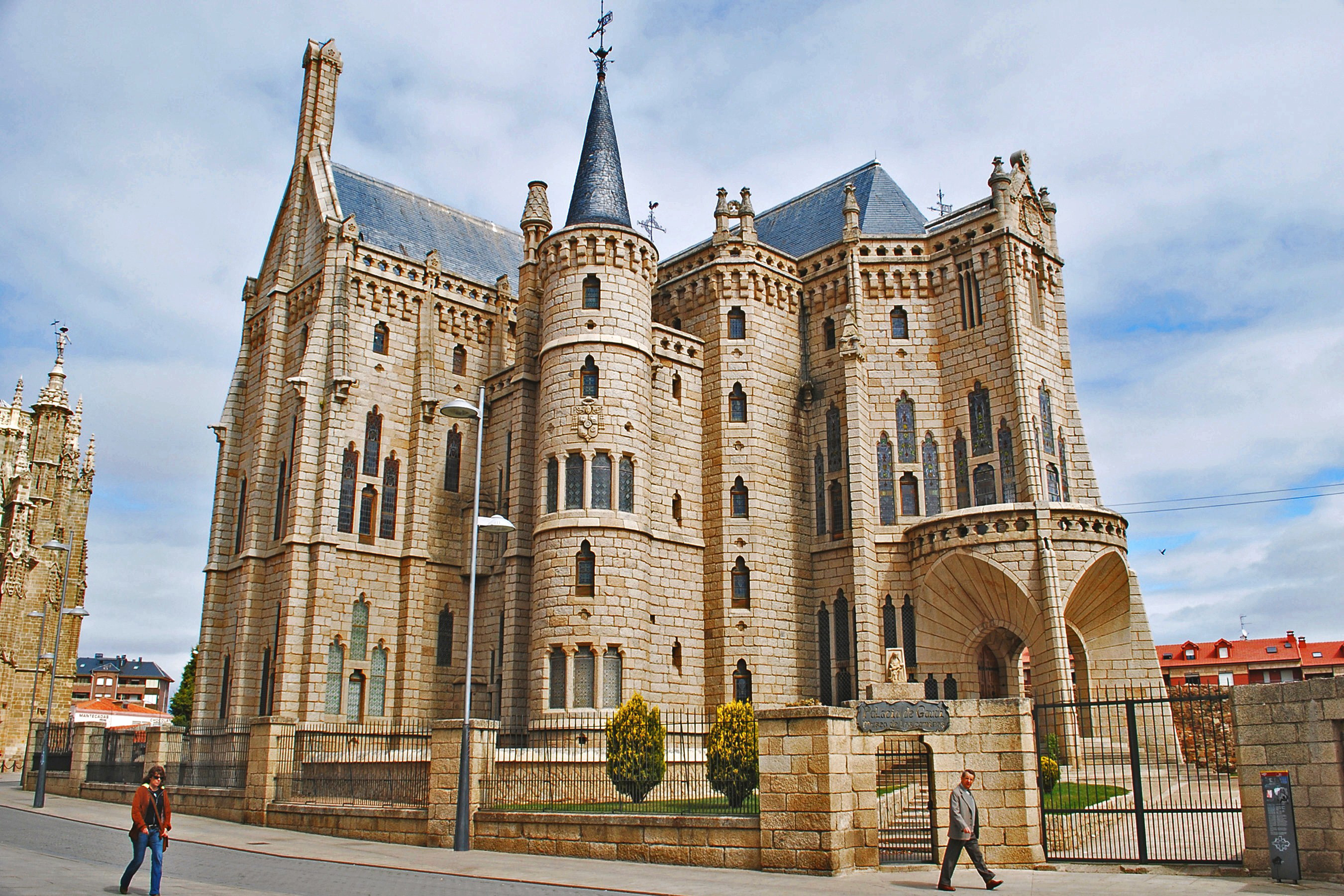
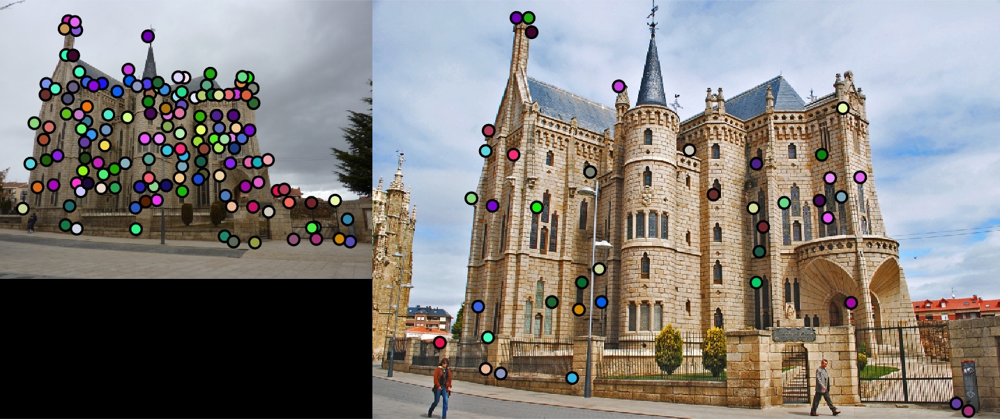
Episcopal Gaudi

Above, we have the three different images we will be focusing on for this project. They are shown in order of expected difficulty.

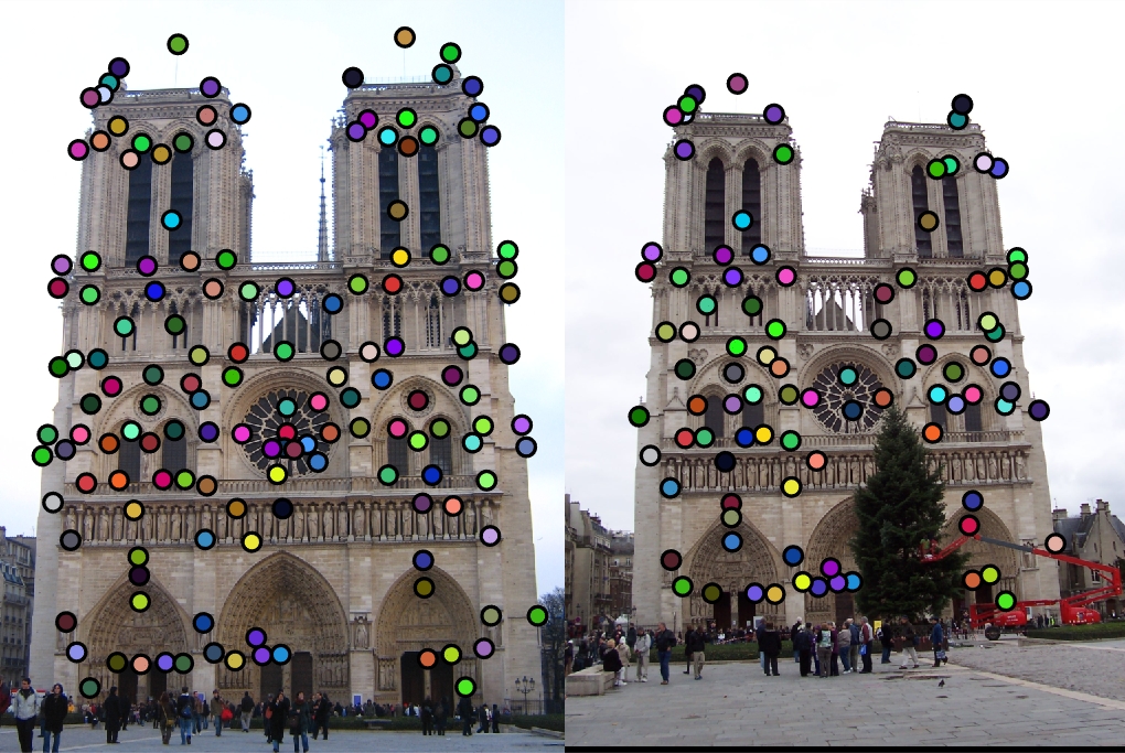
Cheat Interest Points and Image Patches

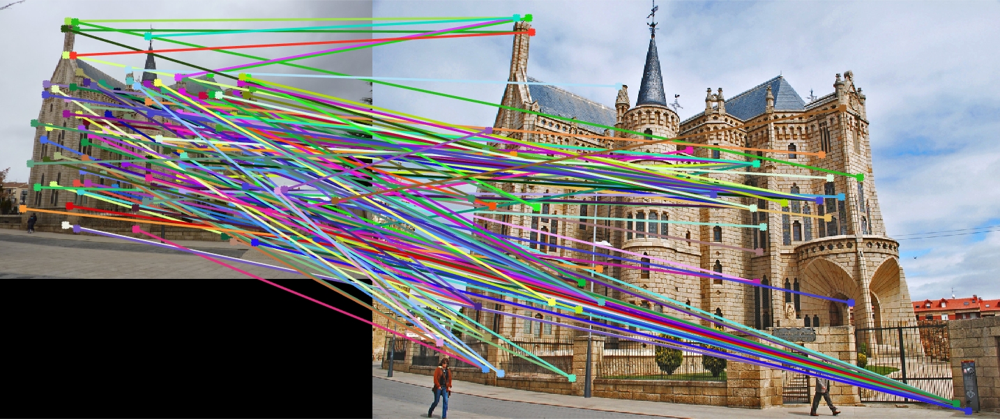
To start with, we will investigate performance when loading predetermined interest points and using 16x16 image patches as our features. That is, we are using the raw pixel values of the patches as our features. Our matching algorithm utilizes the Nearest Neighbor Distance Ratio. We look at the 2 nearest neighbors of an interest point and use the ratio of the nearest neighbor distances to produce confidence values for each match. This is how we get our top 100 matches.

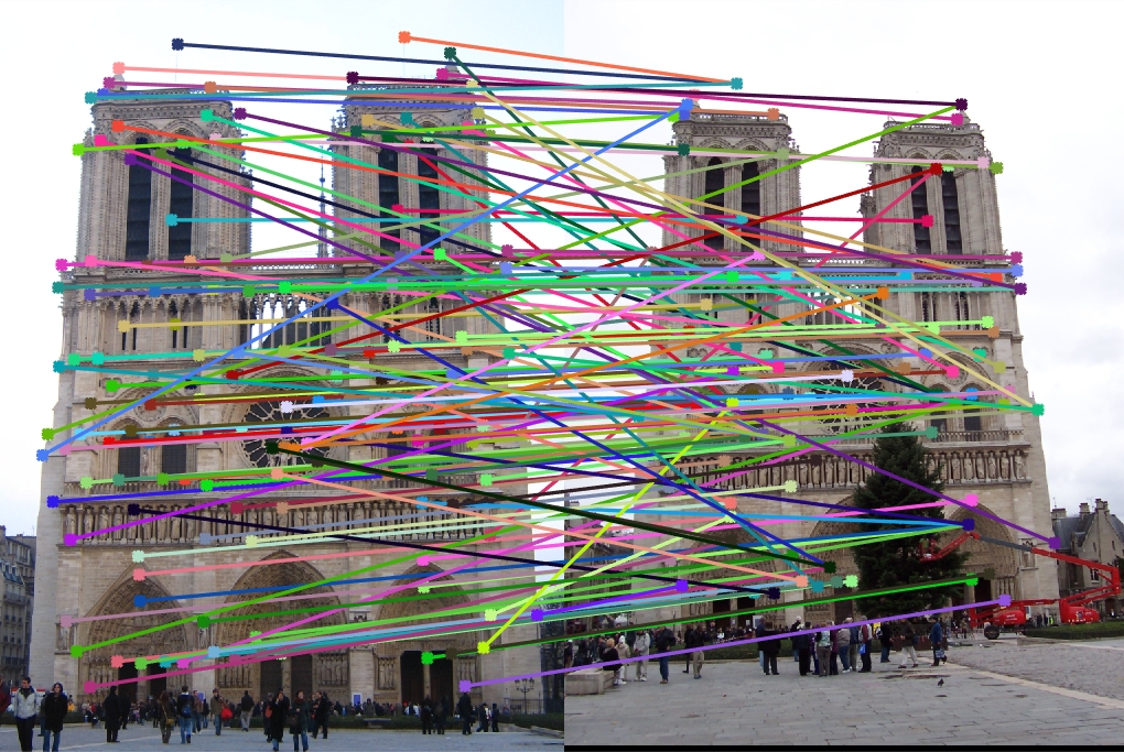
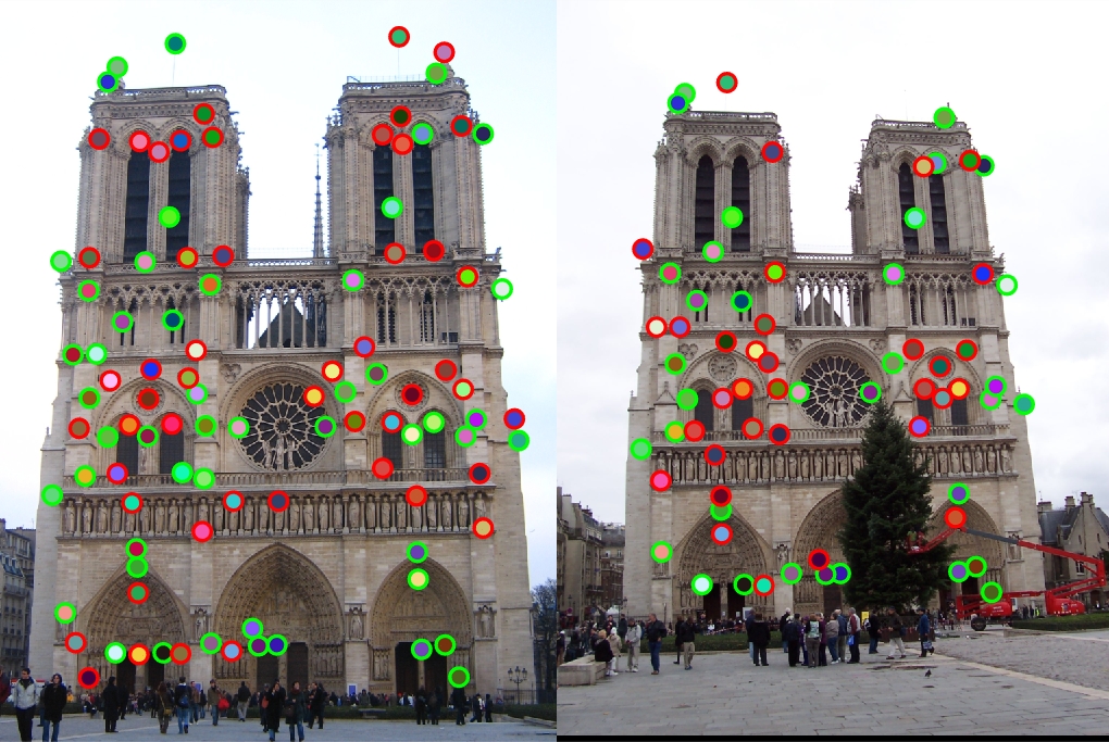
Above, we have performance on the Notre Dame images. We achieve an accuracy of 50%. This accuracy is mediocre but should be expected with such a naive implementation.

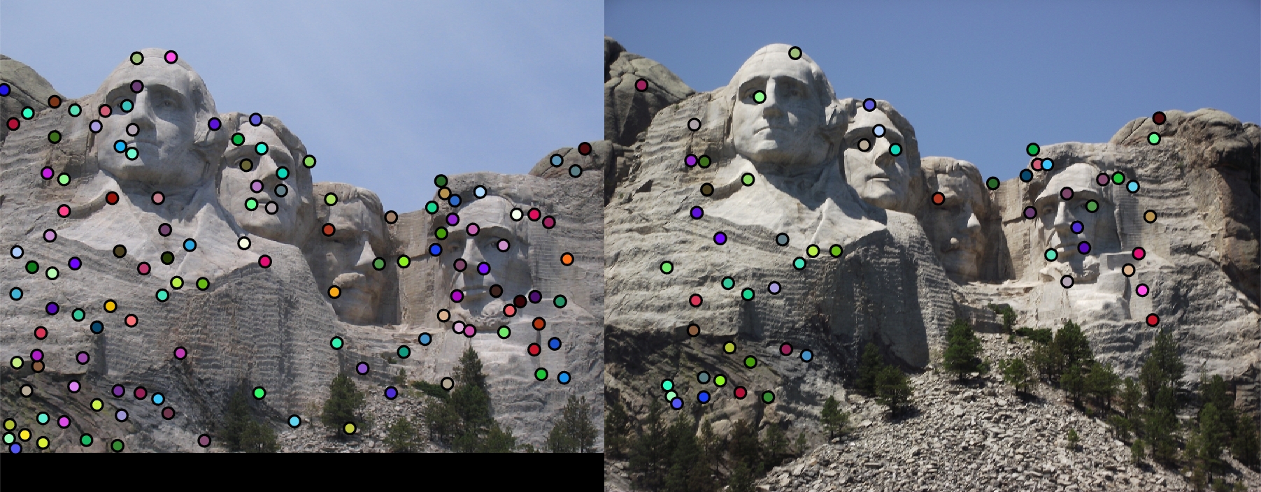
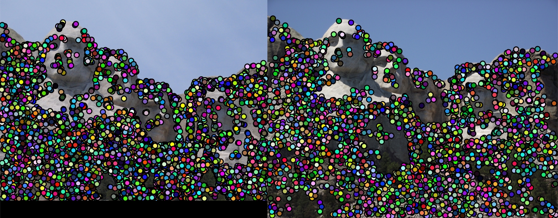
With Mount Rushmore, we suffer a bit more and get a 25% accuracy. When visually comparing the images, we can see that the coloring of the images vary. We would expect this to have a negative effect on the performance when using image patches.

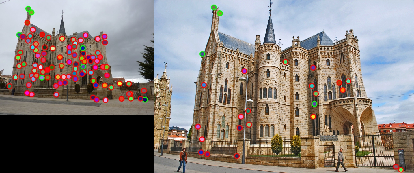
Gaudi proves to be the most difficult image to match. Here, we achieve an accuracy of 8%. The coloring of the images are drastically different, and the scaling doesn't help either.

Cheat Interest Points and SIFT

Now we utilize a more sophisticated feature technique: SIFT. With SIFT, we create orientation histograms of image gradients for subcells of the images. The idea is that this approach is more resistant to negative effects of scaling, coloring changes, and orientation differences. For example, ideally, the gradient will be similar even if the colors are different due to different weather conditions.

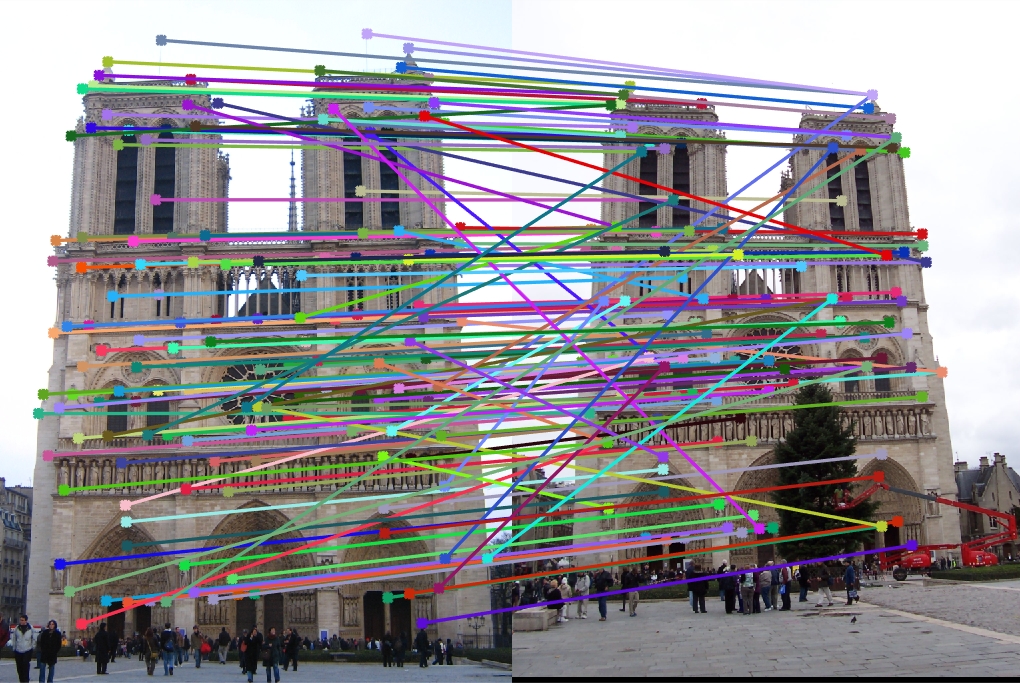
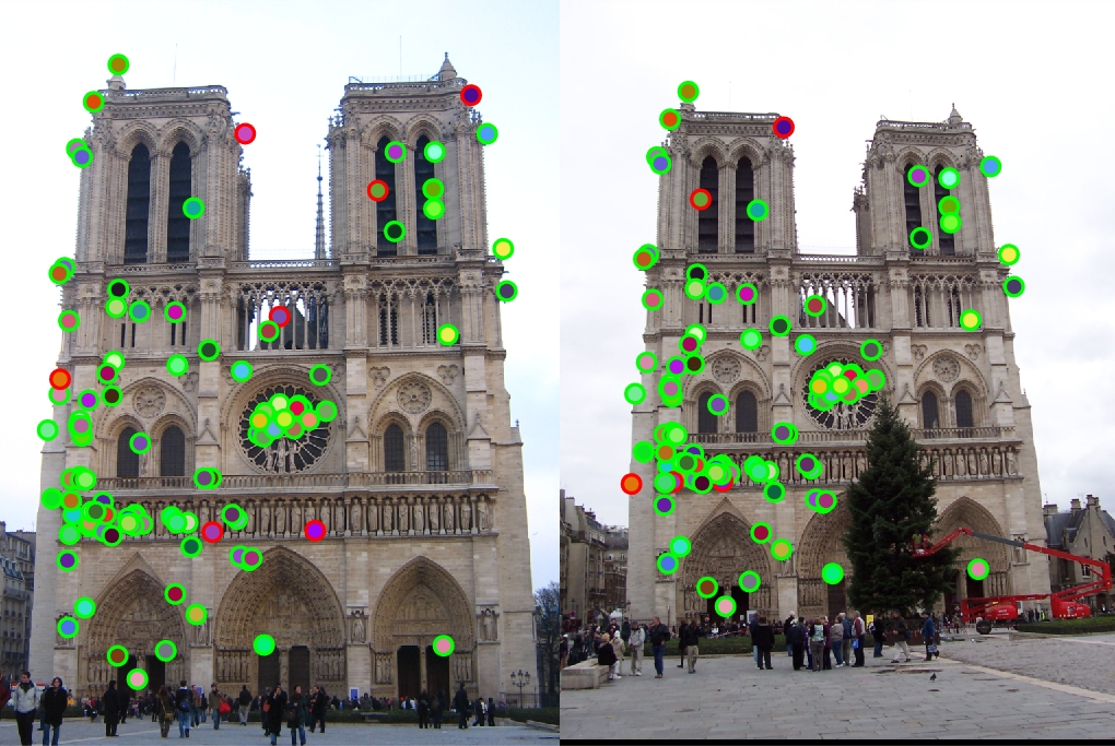
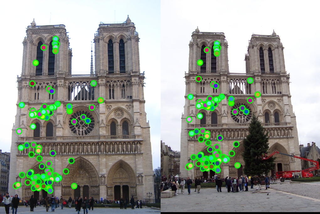
SIFT lets us achieve 75% on Notre Dame. Interestingly, we pick up a lot more matches in the center of the image where the gradients are strong and distinctive. We also see this in places where the building comes to a point. Clearly, SIFT is doing something right.

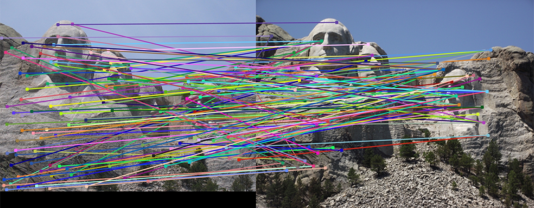
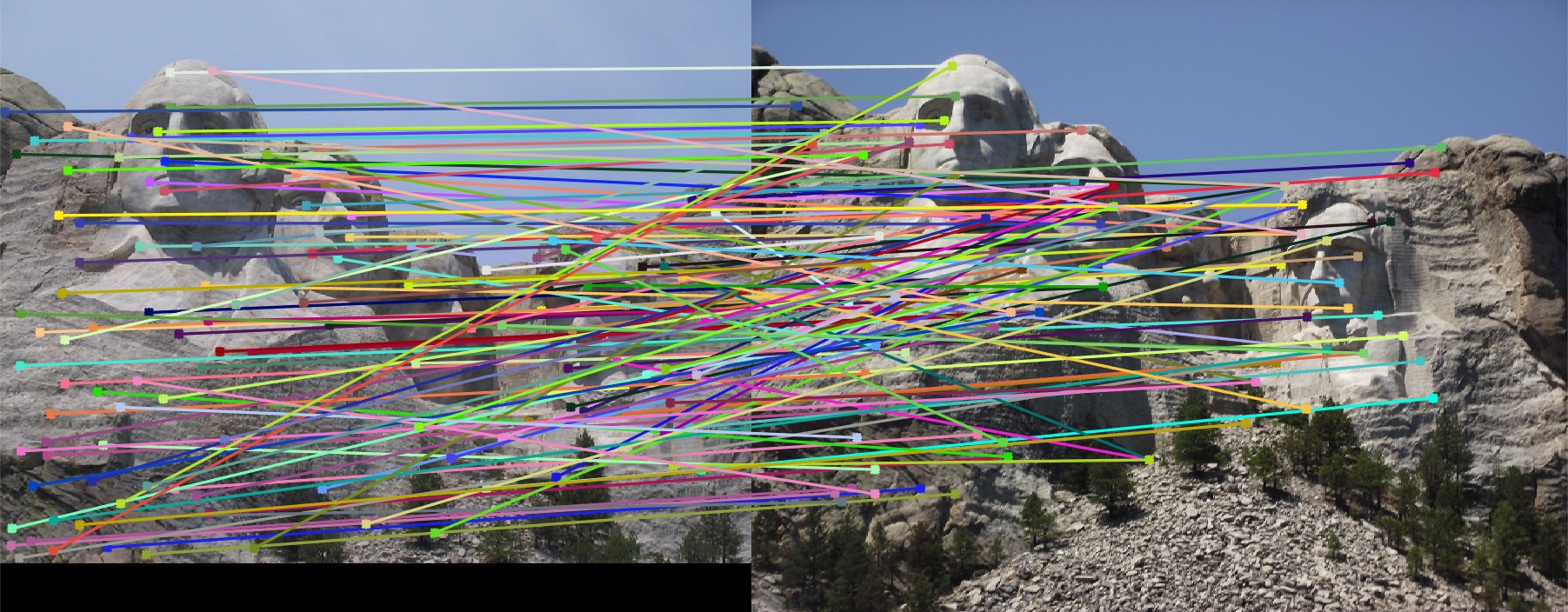
Mount Rushmore also increases to 42%.

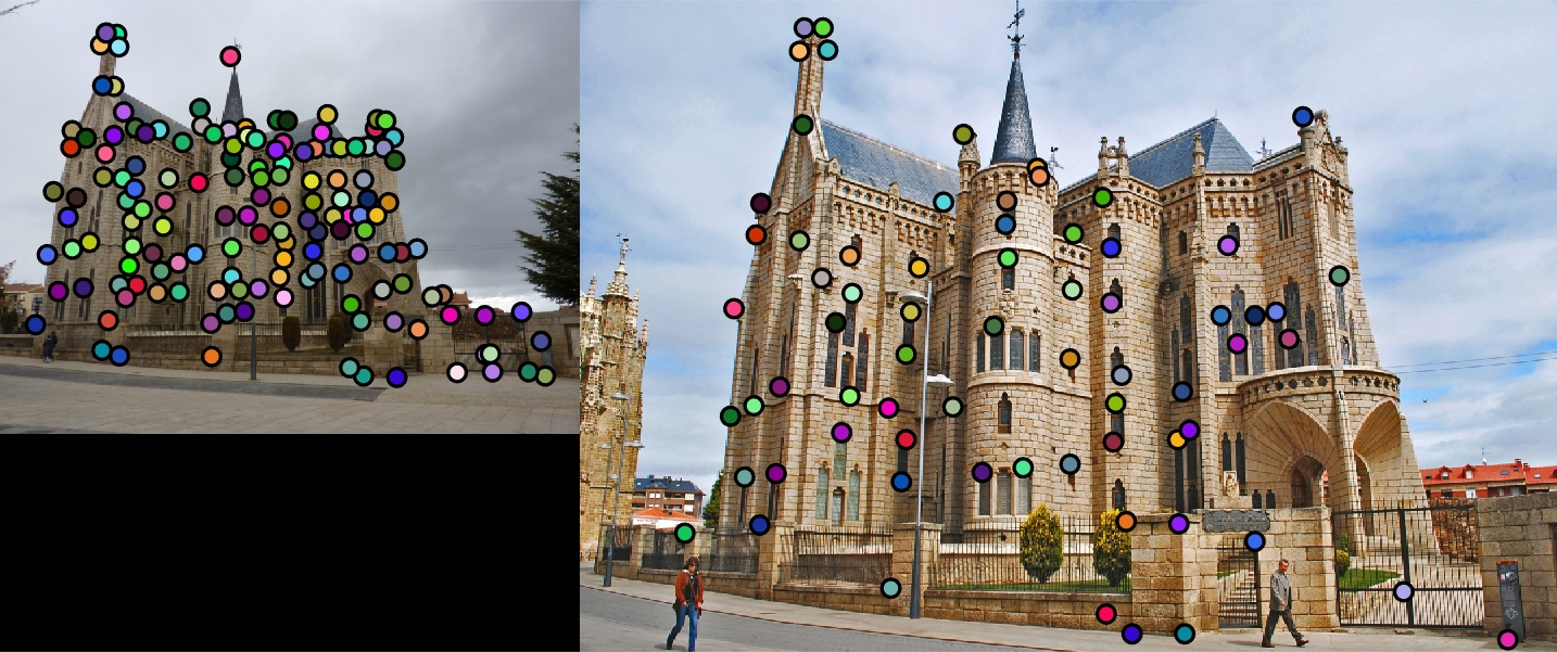
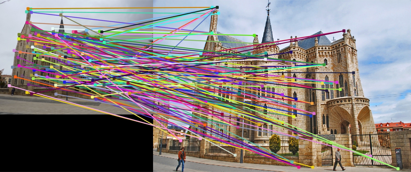
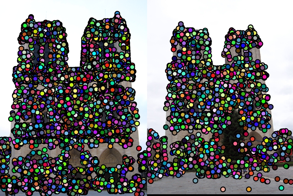
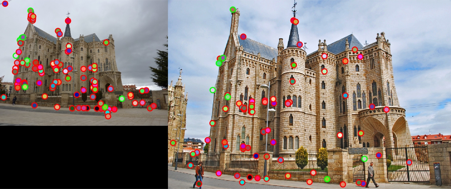
Episcopal Gaudi manages to increase to 18% accuracy. Interestingly, most points are found on the left side of the image. This is perhaps where our images are most consistent.

Harris Corner Detector and SIFT

In this section, we have implemented a Harris Corner Detector. Now we will be finding our own interest points in each image. This is the completed pipeline.

Free Parameters

Now that we have the full pipeline, let's talk about the free parameters. There are a considerable number of things to tweak when trying to configure for the highest accuracy. It took quite a bit of tuning to achieve the accuracies we will visit below. Here are some of the free parameters and notes on how the parameter affected the tuning process:

Method of finding image gradients (filtering with a sobel filter or derivative of Gaussian): a sobel filter tended to perform 2% points higher. The Guassian approach required a much smaller corner threshold of 0.000000000000000001 for 91% Notre Dame/97% Mount Rushmore
Guassian blurring (standard deviation and size) of gradients: 3x3 worked best with a sigma of 10 (sigma did not affect results that much, while differing sizes seemed to mostly negatively impact results)
Harris corner threshold: big boost from tweaking this: .005 = 81%, .000425 = 93%. Lower threshold values worsened accuracy; this was a sweet spot. We take only corners with corner values higher than this.
Size of neighborhood for non-maximum suppression: 5x5 was definitely superior
Value of alpha in Harris corner formula: .04 was best by a few % variation
Nearest neighbor distance threshold: I found that no threshold (i.e. a very large one such as 10) performed just fine
SIFT feature size: larger feature sizes (>16) tended to improve accuracy
Local feature power raising: .3 was the sweet spot; it improved accuracy a lot!
Method of weighting orientation histograms: Just added the magnitude to the bin; weighting the orientation very slightly improved accuracy (by a few %)

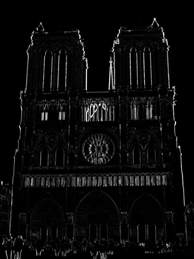
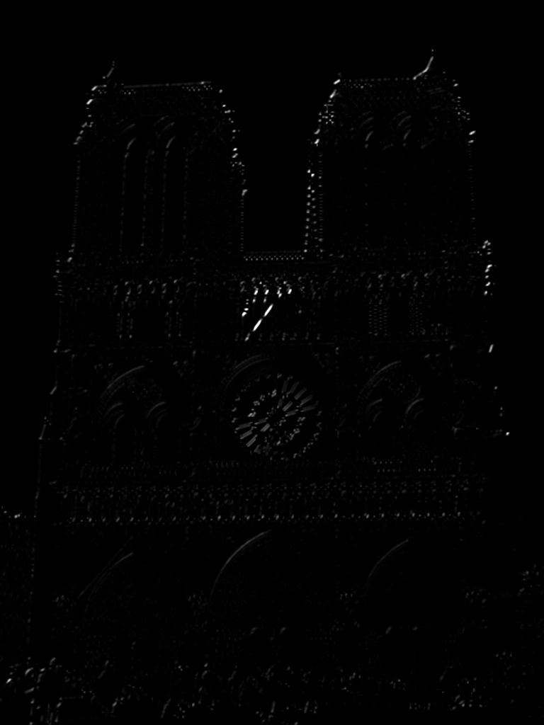
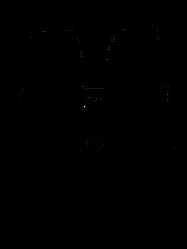
% Harris Corner Detector Formula
corners = gIx2 .* gIy2 - (gIxy .^ 2) - alpha * (gIx2 + gIy2) .^ 2;

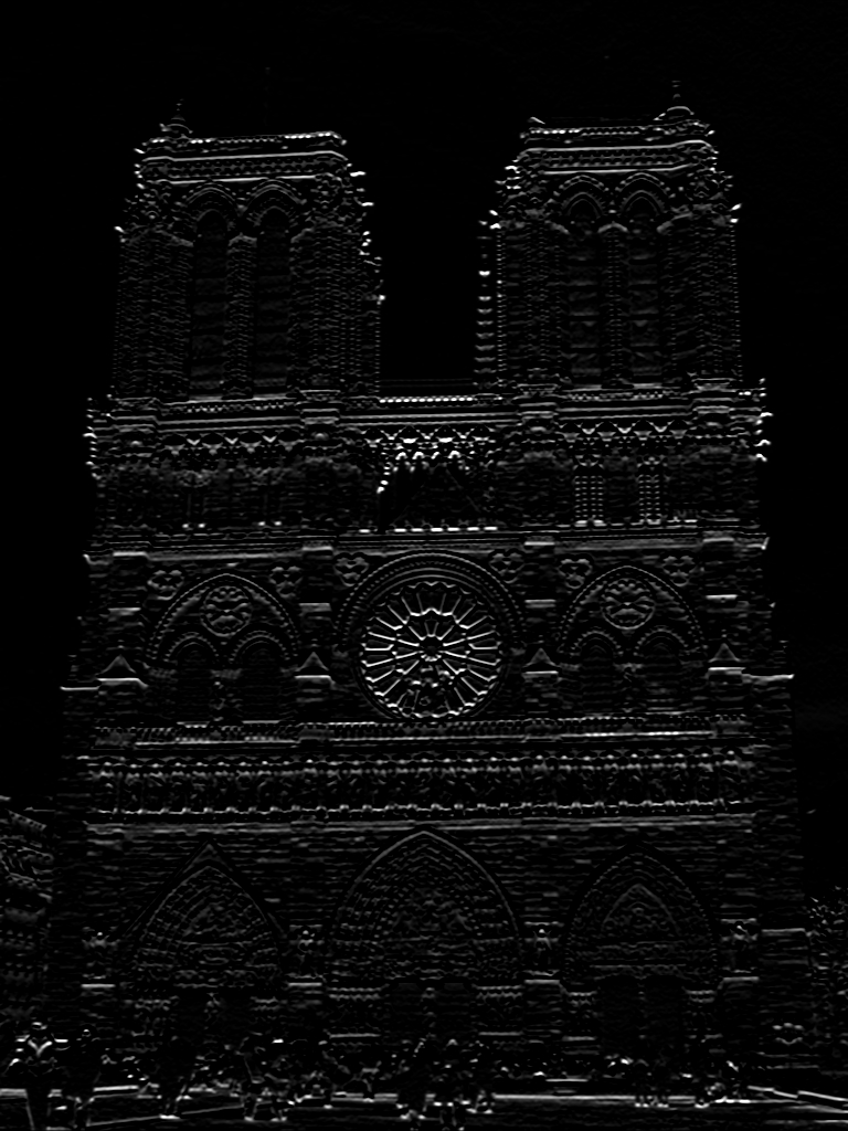
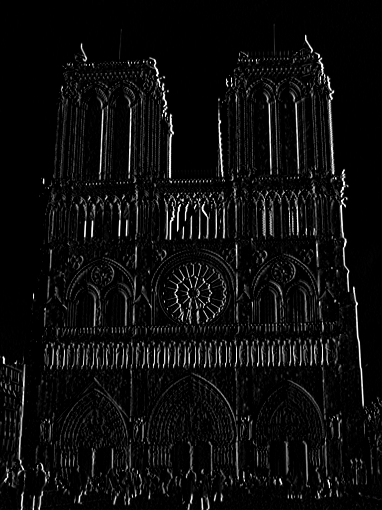
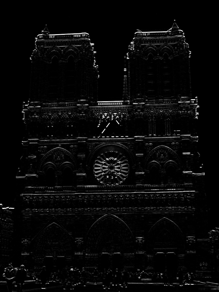
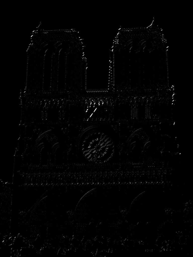
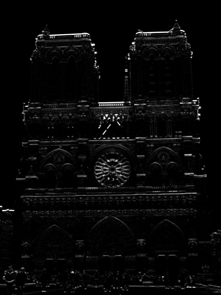
Above is our final corner detector formula that we want to compute. Let's take a look at the the individual steps of the Harris corner detector.

First, we find the x and y gradients of the image, respectively. Notice that the x gradient identifies horizontal edges and the y gradient identifies vertical edges.

Next, we square the elements of the matrices to intensify the gradients. As you can see, it becomes much more clear where our edges lie.

Our Ixy term is just the product of our x and y gradients. Now we can clearly see diagonal gradients.

We pass the x, y, and xy gradients through a gaussian filter to smooth out the edges so they are more pronounced.

After passing our results above through our Harris Corner formula, we get a faint image made up of our detected corners (first image). Some pixels are difficult to see because they have such low values. We perfom some non-maximum suppression by first finding max values in neighborhoods (second image). In this case, our neighborhoods are 5x5, which seemed to peform the best.

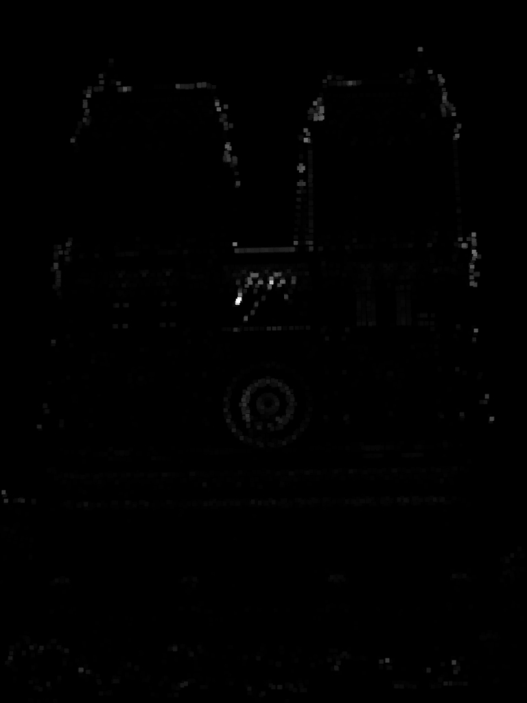
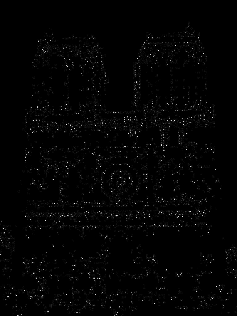
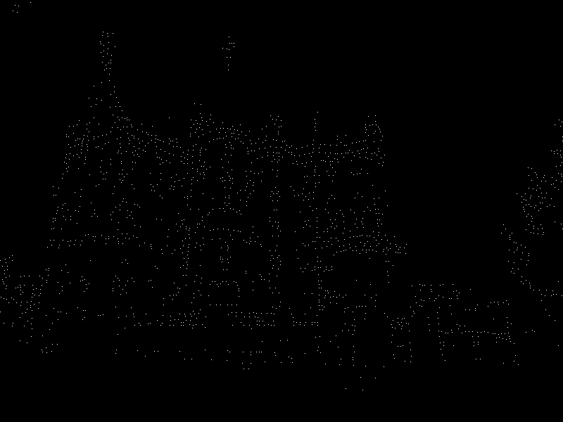
Next, we retain only the max values in the neighborhood and threshold the corner scores so that we only get the strongest corners. Our final result shows us our identified corner interest points. We can clearly see an outline of our original image which is a good sign that the detector is working.

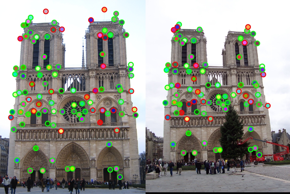
Above, we have performance of the Notre Dame images. Since there are so many interest points, I have excluded the arrows visualization since it gets quite messy. We get around 3500-4100 interest points with this approach. We achieve an accuracy of 93% which is quite impressive, really. We see a huge accuracy boost from using our corner detector, but the real boost was from tweaking the free parameters within the detector.

One important SIFT design decision relates to the bins of the orientation histogram. Originally, my bins split the cardinal directions into two bins. For example, 89 degrees was in bin 1 and 91 degrees was in bin 2. After some thought, I considered that this might have some negative implications on the SIFT features in the case of slight orientation changes. Since our world has so many horizontal and vertical orientations, I think it is important to not split the bins on the cardinal directions (including NE/SE/SW/NW) by rotating the bins by 22.5 degrees. With this new histogram, an 89 degree gradient will go in the same bin as the 91 degree gradient. I think this would definitely make a difference in the case of slight image orientation differences due to the pervasiveness of these types of orientations. This raised the performance of Notre Dame from 88% to 93%.

% SIFT histogram binning. dir is in [0, 360]
% N/NE/E/SE/S/SW/W/NW are at the center of the buckets
bucket_index = floor((dir + 22.5) / 45) + 1;
if (bucket_index > 8)
    bucket_index = 1;
end

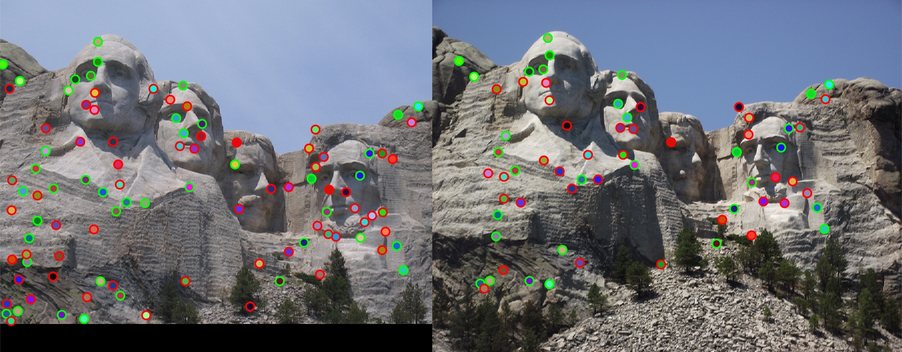
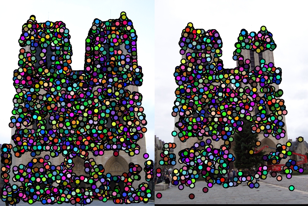
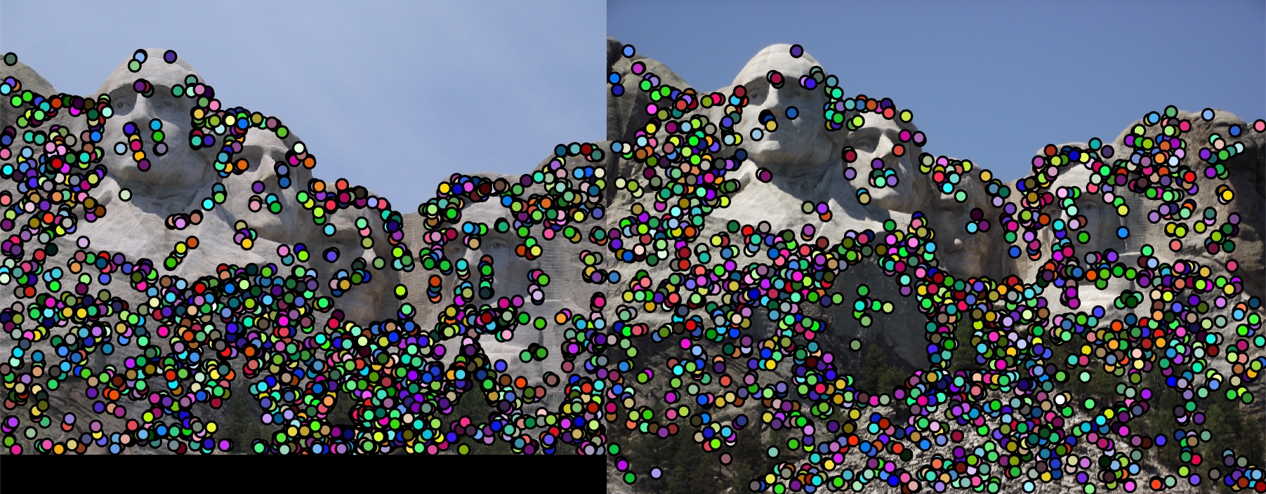
Now we move to Mount Rushmore. Above, we see the interest points that were found. It it not immediately clear what the original image even is! We get a significant number of interest points (over 10,000), but filter down to consider only around 4700-4800 at no hit to accuracy.

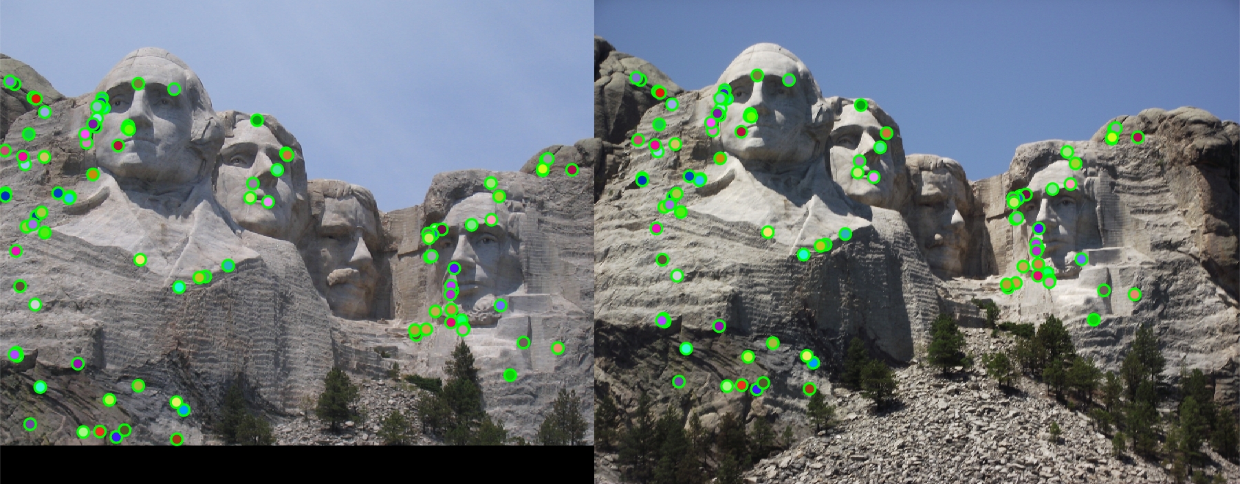
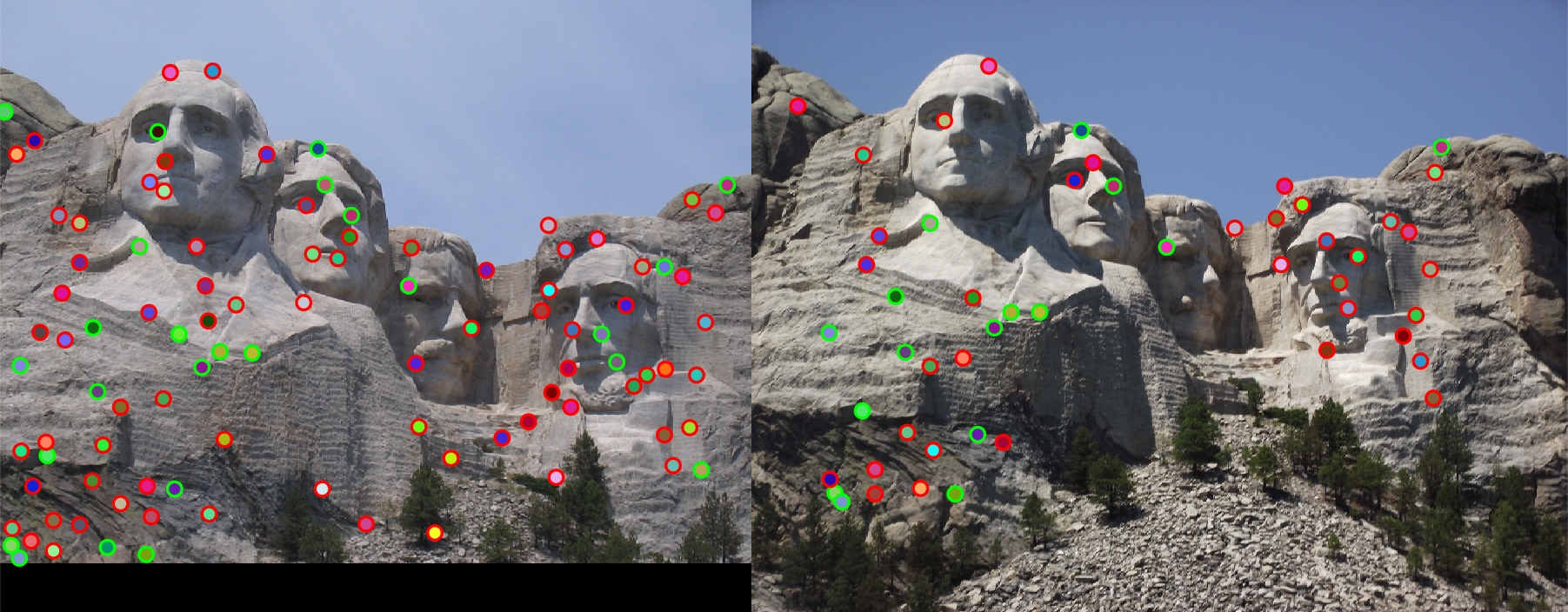
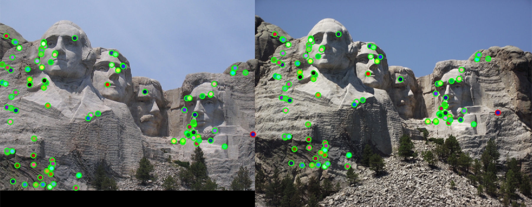
We manage to achieve a 99% accuracy on Mount Rushmore. One would think that this task would be quite difficult due to the seemingly similar rock face. However, it is quite clear from these results that the rock face actually has quite distinctive gradients from the shadows and varying surface gradients. These variations definitely help us identify the interest points and match them across images.

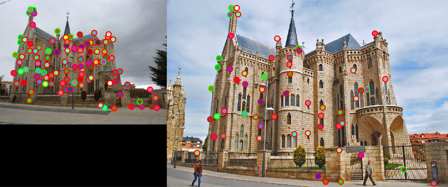
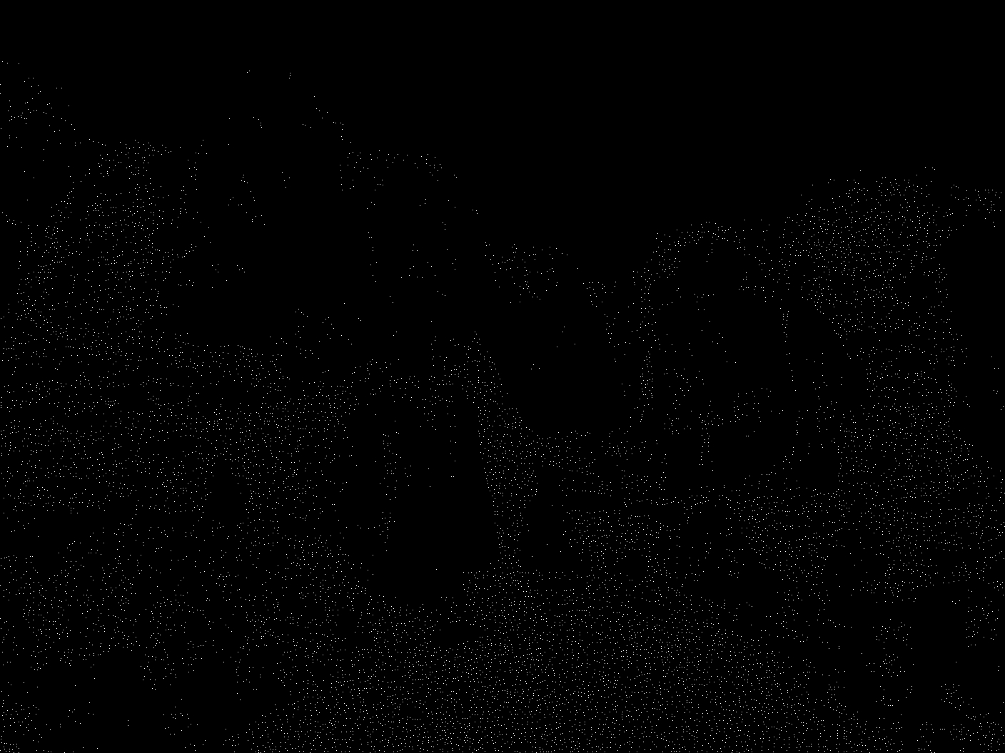
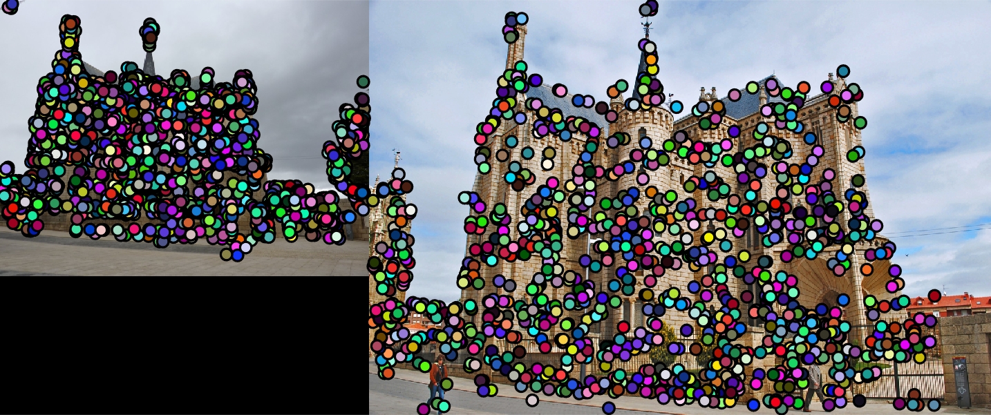
Our final Episcopal Gaudi interest points do well at outlining the building.

Our performance actually drops to 8%. It would appear that our coner detector is the cause of this performance drop. It would seem that since the images are so different color-wise, the corners being detected are not the same, giving us poor performance. Our left image nets us around 1600 interest points, while our right image produces around 10,000 points (but we filter down to around 4900). This imbalance is clearly a part of our problem.

Maximizing Accuaracy

Earlier, we saw that we could get an accuracy of 93% on the Notre Dame image. What about 100%? The above images show that by increasing our SIFT feature size from 16 to 36, we can achieve a 100% accuracy. It makes sense that increasing our feature size would improve our accuracy especially when using two images which are so similar. At a larger size, we start to average out to features that are more similar between the images since we start to cover more overlapping image area. We just have to realize that larger features means more processing and more memory (although that is not noticeable in this example).

I was also curious how hard it would be to bump up Rushmore's accuracy from 99% to 100%. A run with 100% accuracy is shown above. I found 3 very easy ways to do so:

Change the sobel filter to use -1 -1 -1 and 1 1 1 instead of -1 -2 -1 and 1 2 1
Use a SIFT feature width of 36
In the final Harris Corner formula, use 2gIx2 instead of gIx2 + gIy2

Of course, these tactics do negatively affect Notre Dame, so these are perhaps just methods to overfit to Mount Rushmore. I was very surprised to see Mount Rushmore perform so well. It seems that final tuning to bring Notre Dame's accuracy to 93% caused Mount Rushmore's accuracy to skyrocket. Does this improve our poor performing Episcopal Gaudi image matching? Unfortunately not. We get a whopping 6% when using a 36 SIFT feature width. No obvious tweaking seemed to improve accuracy of this image matching; I imagine high accuracy on this image would require more sophisticated features and corners.

Speed

Another factor to consider is the speed of the image matching

The project definitely spends the most time in the 1) interest point matching and 2) graphing phases. While we can't do much about 2), 1) was an easy slowdown to address. I saw a pretty good speedup by using Matlab's knnsearch. Here we measure the time taken to start the visualization process (indicating that we have completed the core pipeline) between the two implementations.

	Naive nn	Matlab knnsearch
Notre Dame	36.191s	9.071s
Mount Rushmore	53.816s	15.991s
Episcopal Gaudi	22.026s	9.802s

After improving the speed of the matching process, most of the time is spent in the get features component. Reducing the feature size from 128 dimensions to something smaller would be something to investigate (although I did not try this here).

Conclusion

Here we have our summarizing table:

	Cheat interest points + image patches	Cheat interest points + SIFT	Harris corner detector + SIFT
Notre Dame	50%	75%	93%
Mount Rushmore	25%	42%	99%
Episcopal Gaudi	8%	18%	8%

It is quite clear from these results that there is no guaranteed method for maximizing image matching accuracy. Even with our core algorithm in place (Harris corners and SIFT), we required significant tweaking and estimating to crank out the highest accuracies. Even with this tweaking, such as in the case of Gaudi, we may not even be improving with every image set. This just reinforces how difficult this task really is.

Graham Wright