Computer Vision Project

Project 2: Local Feature Matching

For this project, the components of a local feature mapping pipeline were developed and tested in Matlab. The first stage of the pipeline was interest point detection, which used a Harris detector to locate strong corner points in each input image. After interest point detection, each point was assigned to a feature vector. The feature vector used SIFT-like features to describe the local image patch around each interest point. Once the features were determined, the interest points were matched between two photos of the same object by determining the Euclidean distance between each feature in both images and using the ratio test to avoid matching ambiguous points. The results showed matching accuracies of over 80% on two pairs of test images. Additionally, PCA was used to significantly reduce the dimension of the feature space while still maintaining high accuracies on both test sets.

Interest Point Detection

For the interest point detection, a Harris corner detector was implemented as the function get_interest_points() in Matlab using the code below:


% Parameters
fsize = 2;
sigma = 1;
alpha = 0.04;

% Get derivative
[Ix, Iy] = imgradientxy(image);

% Square derivatives
Ix2 = Ix.^2;
Iy2 = Iy.^2;
IxIy = Ix .* Iy;

% Filter with Gaussian
f = fspecial('gaussian', fsize, sigma);
Ix2 = imfilter(Ix2, f);
Iy2 = imfilter(Iy2, f);
IxIy = imfilter(IxIy, f);

% Compute cornerness
har = Ix2 .* Iy2 - IxIy.^2 - alpha * (Ix2 + Iy2).^2;

The get_interest_points() function computes the gradient of the image in the x and y directions. It then computes each of the squares of the derivatives (entries in the Harris matrix) and filters these with a Gaussian for smoothing. The Harris cornerness measure is then computed as the determinant of the Harris matrix minus the trace of the matrix times an alpha parameter. Each of the parameters for the algorithm were determined empirically by tuning them to achieve the highest accuracy on the Notre Dame image set. The result of this algorithm is a cornerness value for each pixel in the image. To extract the best interest points from the cornerness score, non-maximum suppression was used according to the code below:


% Cornerness threshold
hthres = 0.01;

% Get connected components
CC = bwconncomp(har > hthres);

% Initialize interest point vectors (equal to # of ccs)
x = zeros(CC.NumObjects, 1);
y = zeros(CC.NumObjects, 1);

% Flatten
[M, ~] = size(har);
har = reshape(har, 1, numel(har));

% Get max cornerness in each CC
for i = 1:CC.NumObjects
    [~, ind] = max(har(CC.PixelIdxList{i}));
    ind = CC.PixelIdxList{i}(ind);
    x(i) = 1 + floor((ind-1)/M);
    y(i) = 1 + mod(ind-1, M);
end

The non-maximum suppression code uses Matlab's bwconncomp() function to identify each connected component in a thresholded version of the cornerness matrix. For each of the resultant components, the pixel with the maximum cornerness is selected as an interest point and its coordinates are added to the output x and y vectors. The figures below show the interest points chosen by the Harris detector for two images of Notre Dame:

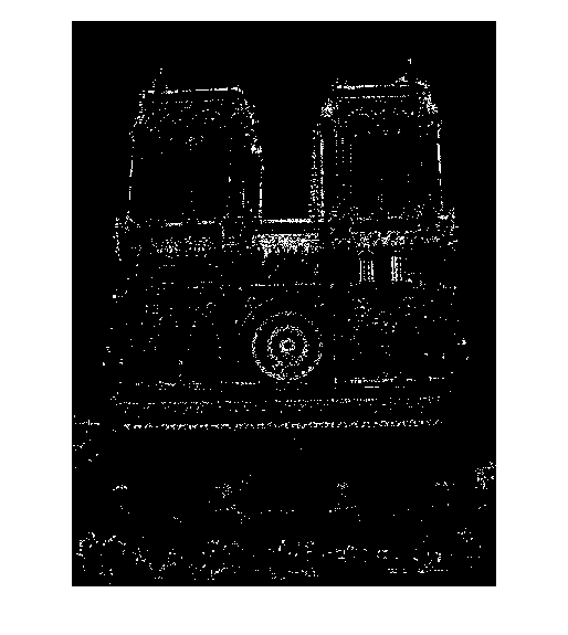
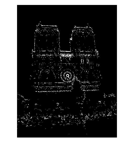
Thresholded Harris cornerness for two images of Notre Dame

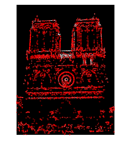
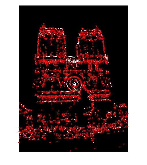
Interest points chosen after non-maximum suppression

Feature Descriptors

After the interest points are selected, each point is described using a SIFT-like feature vector. This was implemented in the get_features() function in Matlab as follows:


% Initialize feature vector
features = zeros(size(x,1), 128);

% Pad image
impad = padarray(image, [feature_width/2, feature_width/2], 'symmetric');

% Make sure x and y are integers
x = floor(x);
y = floor(y);

for i = 1:size(x,1)
    % Get feature_width x feature_width image patch
    xinds = x(i):x(i)+feature_width-1;
    yinds = y(i):y(i)+feature_width-1;
    patch = impad(yinds,xinds);

    % Compute the gradient in x and y for the image patch
    [Gx, Gy] = imgradientxy(patch);
    [Gmag, Gdir] = imgradient(Gx, Gy);
    
    % Multiply Gmag by a Gaussian
    Gmag = Gmag .* fspecial('gaussian', feature_width, feature_width/2);

    % Create histogram in each of 16 cells - bins are 45 degree increments
    for j = 1:4
        for k = 1:4
            % Get subpatch within this cell
            cindsx = feature_width/4*(j-1)+1:feature_width/4*j;
            cindsy = feature_width/4*(k-1)+1:feature_width/4*k;
            cdir = Gdir(cindsx, cindsy);
            cmag = Gmag(cindsx, cindsy);

            % Divide subpatch of Gdir by 45 degrees and round to get orientation
            cdir = mod(round((cdir+360)/45), 8);
            
            % Create histogram - add Gmag to index specified by above
            featureind = reshape(((j-1)*4+k-1)*8+cdir+1, [1,numel(cdir)]);
            features(i, featureind) = features(i, featureind) + reshape(cmag, [1,numel(cdir)]);
        end
    end
end

% Normalize features
features = features .^ 0.3;
features = normr(features);

After initializing the feature vector, the image is padded by half the feature width in case any of the features lie very close to the edge of the image. Then for each feature, a feature_width x feature_width patch is taken with the interest point at the center. The gradient magnitude and direction are then computed for this patch, and the gradient magnitude is multiplied by a Gaussian with a standard deviation equal to half of the feature width to de-emphasize pixels far from the interest point. The image patch is then divided into a 4 x 4 grid of cells. In each cell, an 8 bin orientation histogram is created by dividing the gradient direction for each pixel by 45 degrees and rounding to the nearest integer. Each "vote" in the histogram is equal to the gradient magnitude times the Gaussian. After all 16 histograms are computed, the features are taken to a power less than one and normalized to improve matching performance.

Feature Matching

To match the features between two images, the match_features() function in Matlab was implemented as follows:


% Ratio of min dist to 2nd min
RT = 1.1; 

% Compute distance
D = pdist2(features1, features2);

% Sort D to get min and 2nd min for each row (with indices)
[Dsort, inds] = sort(D, 2, 'ascend');

% Use ratio test to remove ambiguous rows
matchrows = find((Dsort(:,2) ./ Dsort(:,1)) >= RT);

% Create matches and confidence matrices
matches = [matchrows, inds(matchrows,1)];
confidences = Dsort(matchrows,2) ./ Dsort(matchrows,1);

% Sort the matches so the most confident ones are at the top of the list
[confidences, ind] = sort(confidences, 'descend');
matches = matches(ind,:);

The code above first computes the Euclidean distance between all feature vectors in each image. It then sorts these points and removes points where the ratio of the minimum distance to the second minimum distance is lower than a threshold. This ratio test helps prevent ambiguous points from influencing the results. Finally, the confidence values (equal to the ratio) are sorted in descending order to select the best matches. The number of matches is capped at 100 in the main project file, so only the most confident 100 matches (or less if there are fewer matches) are retained.

Results

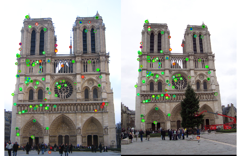
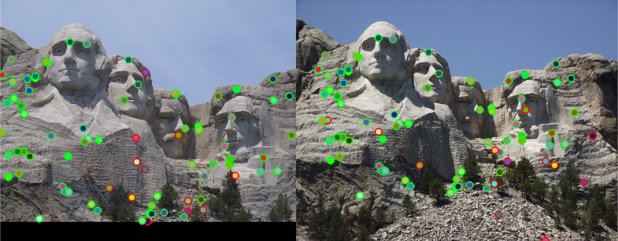
The local feature matching pipeline was tested using three pairs of images of the same object (Notre Dame, Mount Rushmore, and Episcopal Gaudi). The matching accuracy for each set of images is shown in the table and figures below:

Object	Matches	Accuracy (%)
Notre Dame	100	83%
Mount Rushmore	84	85%
Episcopal Gaudi	10	10%

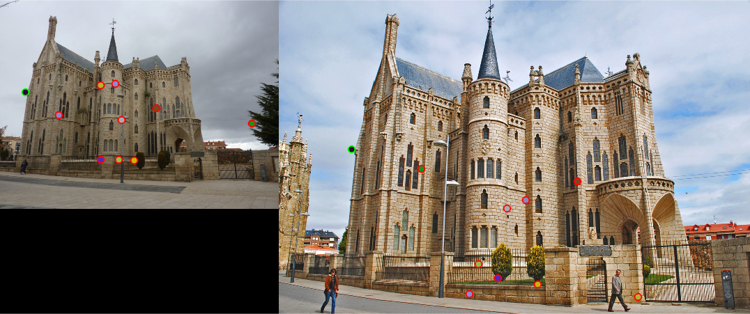
Color coded matches between images for each of the three test sets

The matching accuracy is over 80% for both the Notre Dame and Mount Rushmore images. However, the Episcopal Gaudi images only have an accuracy of 10%. This is likely due to differences in scale, lighting conditions, and orientation between the two images. The matching accuracy is also affected by the number of matches used because selecting only the most confident matches generally yields better results. For the Notre Dame images, taking the top 100 matches produces an accuracy of 83%, while taking the top 50 matches increases the accuracy to 88%. Similarly, the Mount Rushmore set has an accuracy of 85% on 84 matches and 94% on 50 matches. On the other hand, images such as Episcopal Gaudi do not produce many matches at all because most points fail the ratio test. In this case, even the most confident matches are not very accurate.

Dimensionality Reduction with PCA

Since the matching process can be computationally expensive, especially for larger numbers of interest points, dimensionality reduction can be used to reduce the dimension of the feature space without sacrificing much performance. One technique that can be applied is Principal Component Analysis (PCA). This algorithm uses Singular Value Decomposition (SVD) to find the eigenvectors of the covariance matrix for a set of data points. It then projects the data onto a subset of these eigenvectors (the ones with the highest eigenvalues) to reduce the dimensionality of the feature space while still maintaining the axes that explain the most significant variance between the data points. The following code uses PCA in Matlab to reduce the dimensionality of the interest point features:


% Get PCA eigenvectors in order of significance
[coeff, ~, latent] = pca([image1_features; image2_features]);

% Find the variance explained by each eigenvector
cumsum(latent)/sum(latent)

% Reduce the size of the feature space
dim = 64;

% Project the image features onto the new feature space
image1_features = image1_features * coeff(:,1:dim);
image2_features = image2_features * coeff(:,1:dim);

To reduce the dimensionality of the feature space, the eigenvectors (coefficients) and eigenvalues (latent) are computed using PCA on the combined set of features from both images. To determine the amount of variance explained by each eigenvector, the cumulative sum of the eigenvalues can be divided by the sum of all eigenvalues. The more eigenvectors used, the more variance will be explained, but the higher the dimension of the resulting space. The size of the reduced space can then be set and each of the two images can be multiplied by the eigenvector matrix to project the features into the eigenspace. For each of the test images, the elapsed time, variance explained and accuracy were measured for dimensionality 128, 64, and 32. The results are shown in the table below:

Object	Dimensionality	Elapsed Time (s)	Variance Explained (%)	Accuracy (%)
Notre Dame	128	1.79	100	83
Notre Dame	64	1.31	76	81
Notre Dame	32	1.15	56	71
Mount Rushmore	128	2.57	100	85
Mount Rushmore	64	1.91	76	79
Mount Rushmore	32	1.73	56	60
Episcopal Gaudi	128	2.73	100	10
Episcopal Gaudi	64	1.45	73	4
Episcopal Gaudi	32	1.29	53	1

As shown in the table above, reducing the dimensionality by half (from 128 to 64) results in only a small decrease in accuracy. In all three cases, this also reduces the elapsed time by over 0.5 seconds which is a significant reduction when compared to the time it takes for 128 dimensions. In theory, reducing the feature space by half should speed up the matching by a factor of two, though this would likely be more apparent for matching large numbers of interest points than for the relatively small number of points tested here. Reducing the feature space to 32 dimensions results in a fairly significant decrease in accuracy. This is likely because the variance explained by 32 dimensions is only around 55% when compared to around 75% for 64 features.

Haley Garrison

Project 2: Local Feature Matching

Interest Point Detection

Feature Descriptors

Feature Matching

Results

Dimensionality Reduction with PCA