Project 2: Local Feature Matching
Get Interest Points
Set the alpha at 0.085, create the two gaussian filters. Both with the size of the width of the features, one with sigma at 1 (default) and one at 2. Find the image gradient on both vertical and horizontal of the smaller gaussian filter, and filter both of them with the input image using imfilter(). Then suppress the edges to reduce noises by setting the pixel values near the edges to zero. Then compute the three images correspond to the outer products of Ix and Iy, and convolve them with the larger gaussian filter. After that, compute the scalar interest measure by using
harris=det(A)-alpha*trace(A)^2=Ixx*Iyy-Ixy^2-alpha*(Ixx+Iyy)^2.
After computing the interest measure matrix, threshold with the average value of the whole harris matrix. Then using colfilt(), find the maximum value within every sliding window, and only keep those that are equal to the maximum in each sliding windows.
The threshold, window sizes in this method is imprtant for finding good features/matches later on. I started with a high threshold which returned less points, and eventually less features/matches. The parameters of the gaussian filters are also important to find strong responses in the corners.
% Gaussian filters
gaussian = fspecial('gaussian',[feature_width feature_width],1);
larger_gaussian = fspecial('gaussian',[feature_width feature_width], 2);
% compute scalar interest measure
% A = [Ixx Ixy; Ixy Iyy]; harris = det(A)-alpha*trace(A)^2;
harris = Ixx.*Iyy-Ixy.*Ixy-alpha.*(Ixx+Iyy).^2;
% sliding window
harris_max = colfilt(harris, [feature_width feature_width], 'sliding', @max);
harris = harris.*(harris == harris_max);
Get Features
Two gaussian filters with mostly the same parameters were used to get features. (Larger filter uses feature_width/2 as sigma) Then find the gradient in vertical and horizontal direction of the smaller gaussian. Fitler them both with the input image. After obtaining the 2 directional images, we calculate the orientation and magnitude of the gradient, which are obtianed by:
orientation=180*atan2(-Iy,Ix)/pi, magnitude=sqrt(Ix^2+Iy^2);
Then we loop through all the cells to fill in the histograms.
Match Features
The matching threshold is set to 0.6 (except for the Episcopal Gaudi example), and k is initialized to 1 for indexing through the matches matrix. We first loop through both of the features lists and find the distances between the indexed features in the two lists by:
% loop through the features of 2 images
for i=1:size(features1,1)
    for j=1:size(features2,1)
% find distance between two features from 2 lists
        dist(j,:)=sum((features1(i,:)-features2(j,:)).^2);
Then we sort the distances with ascending order to find the closest features. After that, the ratio of the nearest neighbors were calculated. If the ratio is less than the declared threshold, it counts as a match and fills in the return matrices.
Image Results
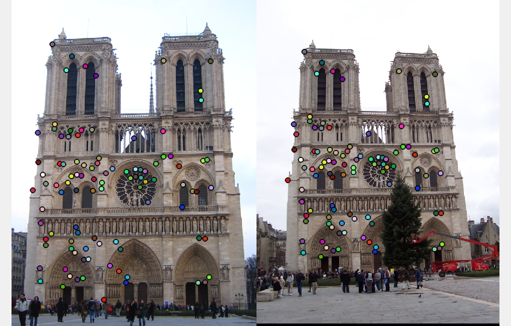
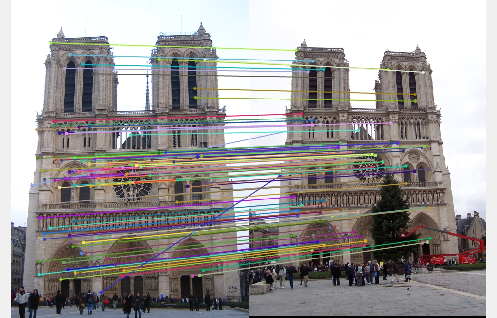
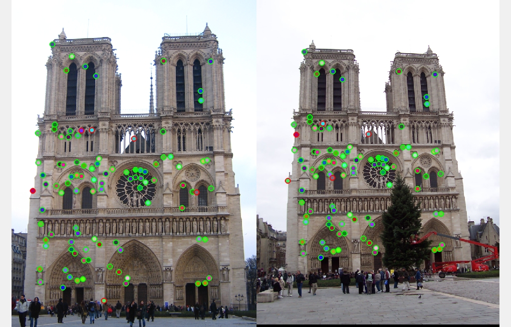
Notre Dame: 94% accuracy, 6 bad matches, 94 good matches. Results are shown below:
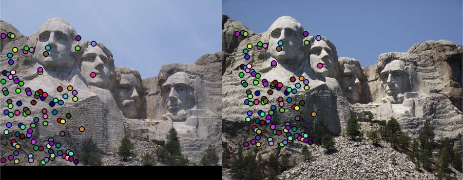
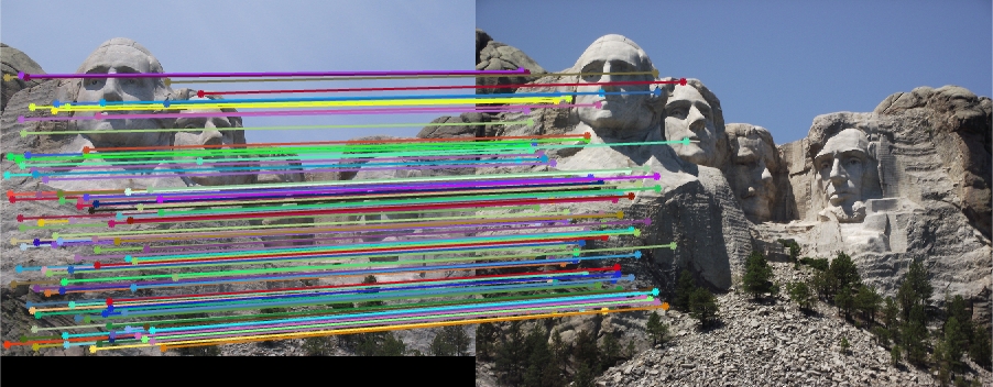
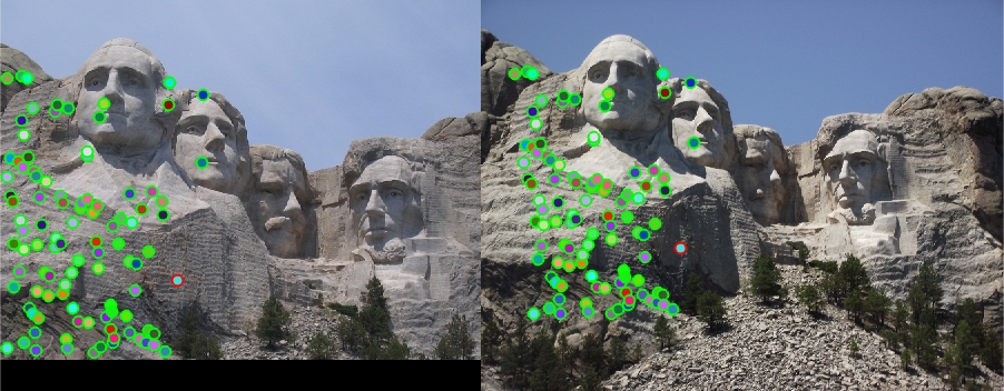
Mount Rushmore: 99% accuracy, 1 bad matches, 94 good matches. Results are shown below:
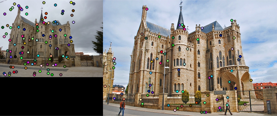
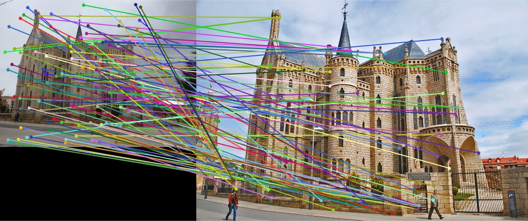
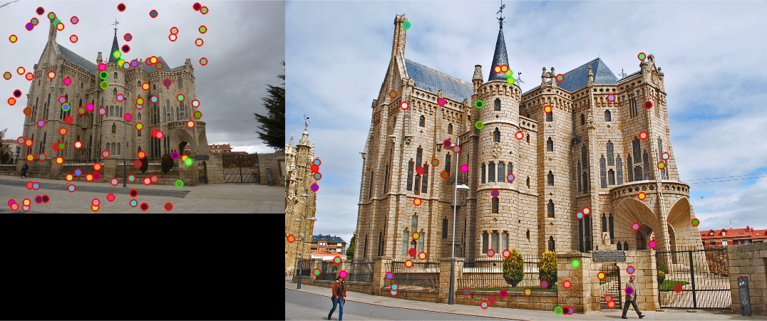
Episcopal Gaudi: The threshold for matching is adjusted to 0.85 to meet the requirement of 100 matches. 8% accuracy, 92 bad matches, 8 good matches. Results are shown below: