Computer Vision Project

Project 2: Local Feature Matching

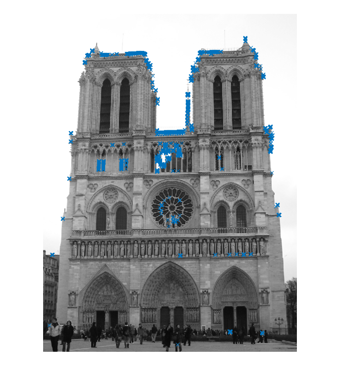
Interest Point Detection (Harris Corners)

Harris corners were used to identify feature points. The parameters used to calculate the Harris score is alpha=0.05 and the threshold is the 99th percentile value.

Local feature description

SIFT-like features were used to describe a given keypoint. The gradients are accumulated in a histogram of 4x4 spatial bins with 8 orientation bins each, resulting in a 128-dimensional descriptor.

%code for SIFT features

[gx,gy] = gradient(patch);
phase = atan2(gy,gx);
bin_x = floor((i-1)/4);
bin_y = floor((j-1)/4);
bin_angle = floor(phase(i,j)*4/pi)+4;

Feature Matching

Feature points from the 2 images are matched according to the Euclidean distance metric between descriptor values. The nearest neighbor distance ratio test was used to pick valid matches.

%code for feature matching

distance(i,j) = norm(image1_features(i) - image2_features(j));
bestMatch(i) = argsort(distance(i))(1);
secondBestMatch(i) = argsort(distance(i))(2);
NNDR(i) = distance(i, bestMatch(i)) / distance(i, secondBestMatch(i));

Extra Credit 1 (Alternative Feature Detector)

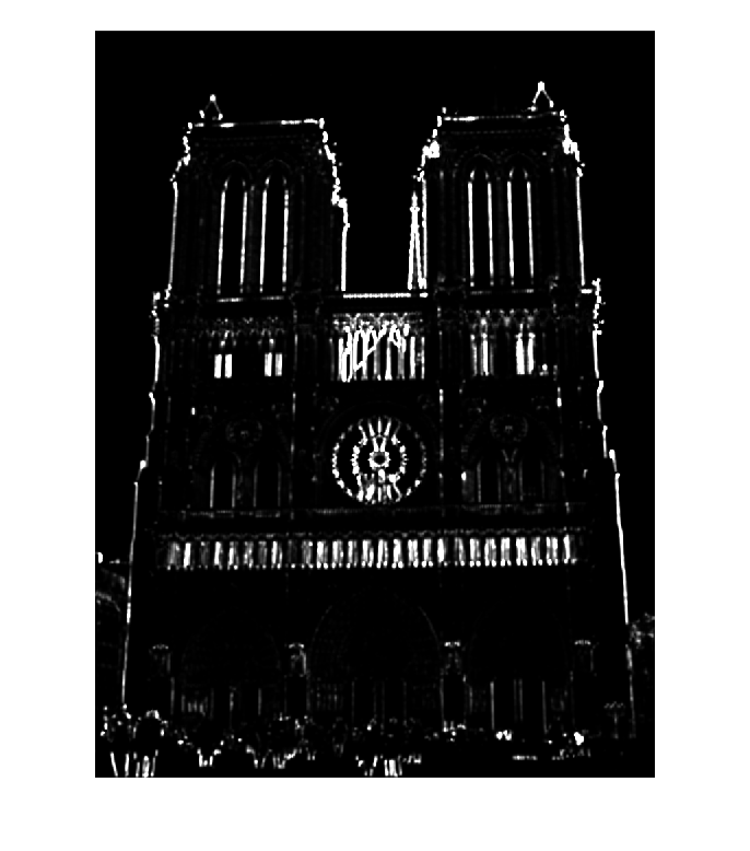
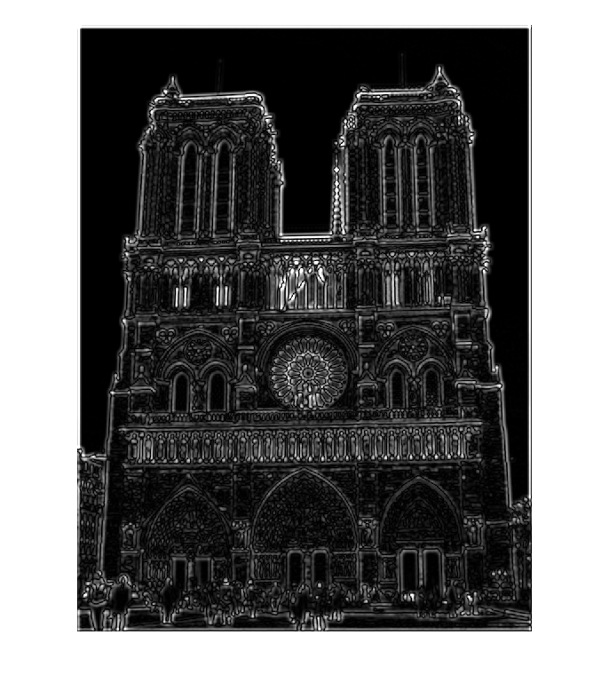
The Laplacian method was used to detect interest points. The Laplacian is estimated using the difference of two Gaussians at different cutoff frequencies. The figures below show the values in the Laplacian matrix and the selected interest points respectively.

Extra Credit 2 (Fast Matching)

A KD-Tree data structure was used to build a database of descriptor values at given feature points. A query descriptor can then be matched to the closest descriptor efficiently using the KD-Tree

%code for KD-Tree

query = features1;
database = features2;
model = KDTreeSearcher(database);
[id,distances] = knnsearch(model,query,'K',2);
matches = [(1:size(query,1))' id(:,1)];

Extra Credit 3 (Dimensionality Reduction)

The technique of Principal Component Analysis (PCA) was used to reduce the dimensionality of the descriptor so that feature matching can be performed more efficiently. A database of 90 image and 3420 descriptors was built to compute a set of basis vectors over the feature space. The results for different number of PCA bases is shown in the table below. As the number of bases decreases, the accuracy decreases but the time to match also decreases.

%code for PCA

[u,s,v] = svd(all_features);
pca_basis = v(:,1:num_bases);
new_features1 = image1_features * pca_basis;
new_features1 = new_features1 / norm(new_features1);

Number of PCA bases	Reconstruction Error (RMSE)	Time to match (s)	Accuracy
128	0	11.38	72%
64	14.45	5.12	67%
32	16.49	2.83	32%
16	17.43	1.21	21%

Extra Credit 4 (Geometric Consistency)

RANSAC was used to estimate a set of transformation parameters between point pairs of the two images and the derived model was used to eliminate inconsistent matches. The transformation accounts for scaling(k), rotation(theta), and translation(Tx,Ty).

%code for RANSAC

for i=1:ransac_iters
	theta,k,Tx,Ty = estimate_param(x1,x2,y1,y2);
	for j=1:numMatches
        dx = k*(cos(theta)*x1(m(1))+sin(theta)*y1(m(1))) + Tx - x2(m(2));
        dy = k*(-sin(theta)*x1(m(1))+cos(theta)*y1(m(1))) + Ty - y2(m(2));
        if (dx^2 + dy^2 < ransac_threshold)
            numInliers = numInliers+1;
        end
		if (numInliers > maxInliers)
			maxInliers = numInliers;
		end
    end
end

The results for 3 image pairs are shown below. Several parameters were adjusted and the best results are reported. For the third test case, the initial accuracy was bad because the image sizes were different. However, when the left image was scaled to be similar to the right image, the achieved accuracy was much better.

Dataset	Good matches	Bad matches	Accuracy
Notre Dame	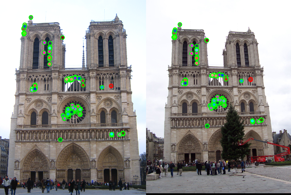496	4	99%
Mount Rushmore	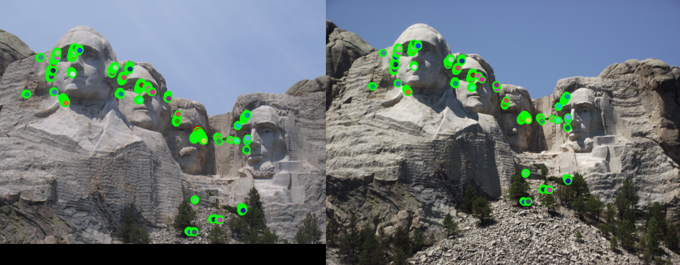986	14	99%
Episcopal Gaudi	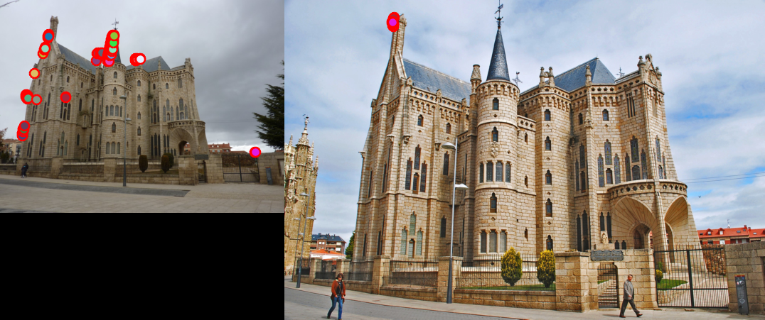0	211	0%
Episcopal Gaudi (rescaled)	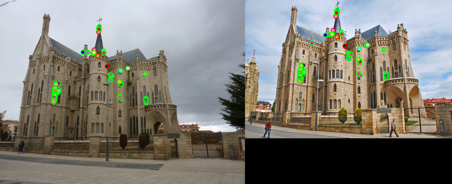321	10	97%

Jingdao Chen