Computer Vision Project

Project 2: Local Feature Matching

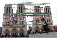
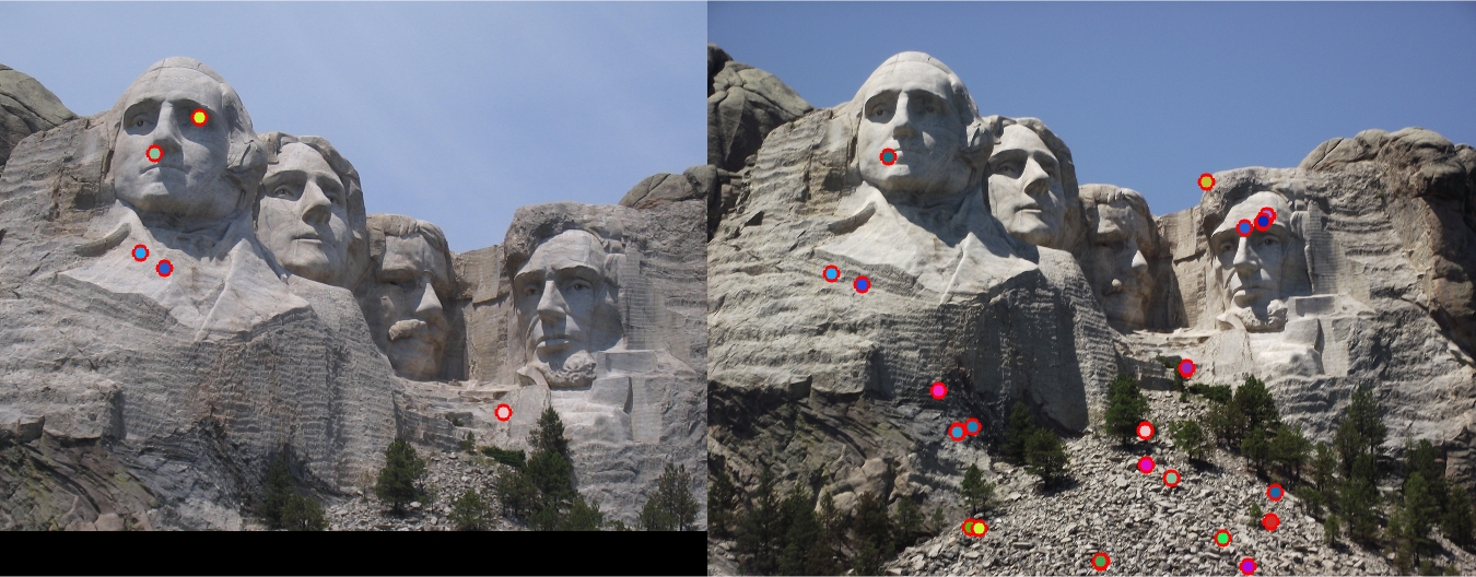
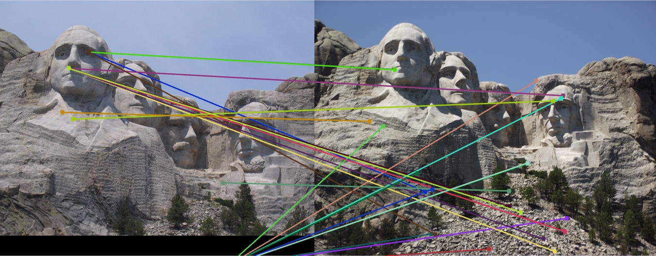
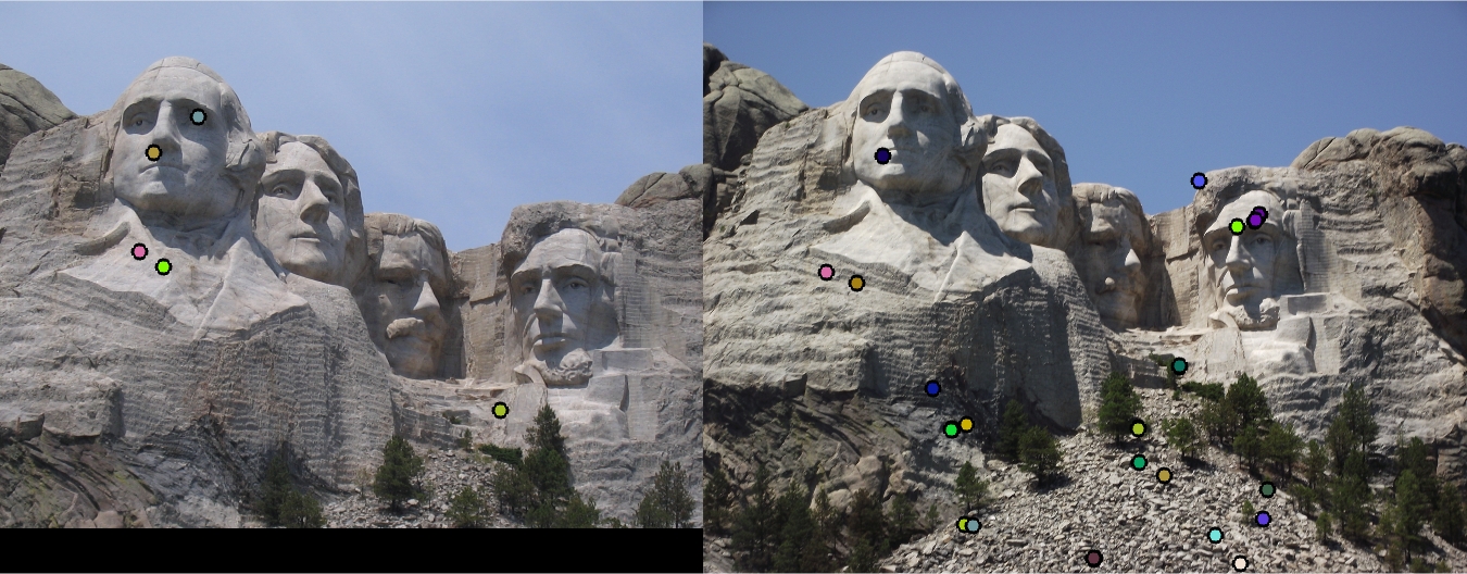
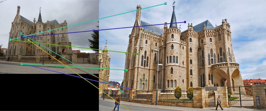
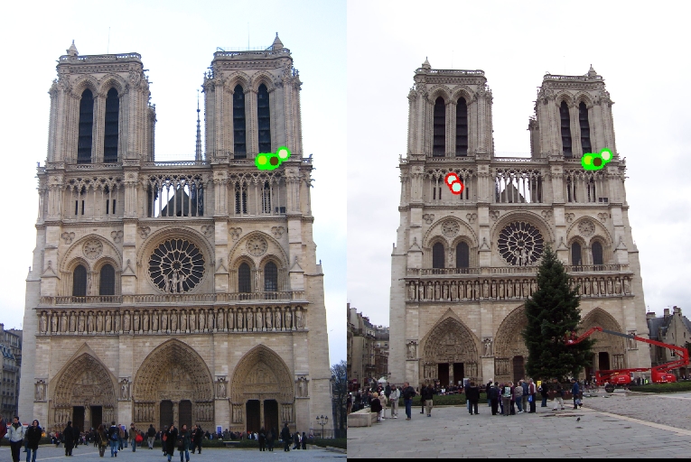
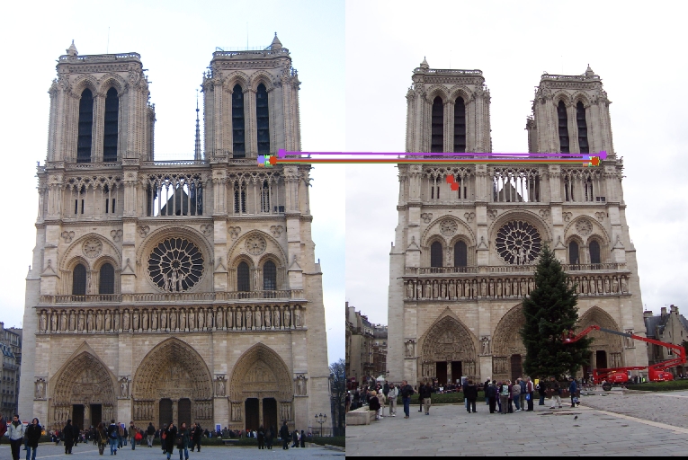
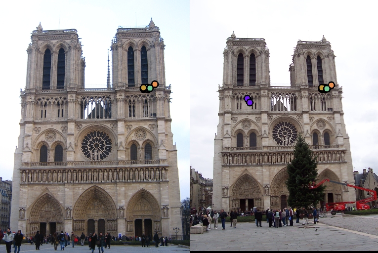
Example of a match.

Introduction of implementation

I implemented orientation invariance and PCA for extra credits.

get_interest_points:
I first blurred the image using 3x3 sigma 1 gaussian, then calculated harris corner response, selected the ones that higher than 0.06 and return. I did not implement scale invariance. Here I found a trick that when the threshold was <= 0.05 or >= 0.07, accuracy was less than 80%. Whereas when it was set to 0.06, accuracy boosted to 86%
I also implemented orientation invarant. See details below.

get_features:
I first blurred the image using 3x3 sigma 1 gaussian, then calculated gradient magnitudes and directions for each pixel. For each interested points, I calculated its 128 sift dimension sift features. I did not implement scale invariance.
I also implemented orientation invarant. See details below.

match_features:
I first calculated the distance matrix where each row corresponds an interested point in figure 1 and each column corresponds an interested points in figure2. Then I sorted the matrix in each row in ascending order so that for each row, its first and second columns were the nearest two neibours, and calculeted NNDR. I also transposed the distance matrix and then did the same steps above. This means that for each interest points in figure1, I calculated its match in figure 2, and for each interest points in figure 2, I also calculated its match in figure 1. It is not a simple duplication, just as "the one who I like may not like me :)". Finally, I return the ones whos NNDR less than threshold.
If the match_features function receives more than 2 parameters, it will go to PCA mode. See details below.

Extra work:

Orientation invarant implementation

get_interest_points: after all interested points achieved, I calculated their orientation according to the 36 bin stratedy. For each key point, a 16*16 window around the it was cut out. All pixels gradient direction were calculated and put in bins. Find the bin with maximal counts, and return its direction for this point.

get_features: first I built a 16*16 relative coordinate 2 * 256 matrix.[(-8,-8);(-7,-8);...(8,-8);(-1,-7);...(7,7)]T. each pair in this matrix correspond to a point in the 16*16 window. Then for each key point, and its orientation, I calculated the corresponding rotation matrix [cos(orientation), -sin(orientation); sin(orientation), cos(orientation)], multiplied the rotation matrix to the 2*256 matrix to get a new 2*256 matrix where each column represents the new relative coordinate of the original point. Then I cut out the gradient directions of the 256 pixels, to perform later sift-like steps.

performance:
no orientation calibration: 102 total good matches, 20 total bad matches. 84% accuracy
with calibrate orientation: 19 total good matches, 1 total bad matches. 95% accuracy

Though the number of matched points became less, accuracy boosted. However, since I did not perform scale invarance step, the performance improvement is not stable and robust;

tips: if you want to test the effects before or after orientation calibration, simply mask or not the first line in get_feature.

PCA implementation

I calculated and saved the projection basis, then modified my match_features to accept parameters to reduce dimension

I also calculated the whole dataset from the provided 3 image pairs, and pooled them together for calculating projection basis. For this test, however, I used projection basis calculated only from the first pair, as the whole projection basis gave a worse performance on the first pair. It makes sense since different images have different properties.

code for calculating projection basis. data_all is from all 3 pairs


co_va_all = (data_all' * data_all)/ size(data_all, 1);
[proj_basis_all,~,~] = svd(co_va_all);
save('proj_basis_all','proj_basis_all')

Performance:
Original 128 features: 45 total good matches, 6 total bad matches. 88% accuracy
Transform 128 features: 45 total good matches, 6 total bad matches. 88% accuracy
Transform 64 features: 69 total good matches, 9 total bad matches. 88% accuracy
Transform 32 features: 102 total good matches, 20 total bad matches. 84% accuracy
Transform 24 features: 127 total good matches, 29 total bad matches. 81% accuracy
Transform 16 features: 148 total good matches, 54 total bad matches. 73% accuracy

Even reduced to 32 dimension, I can still get 84 acccuracy. More surprisingly, after dimension reduction, I get more matched pairs. This means more pairs get NNDR smaller than 0.7 threshold in my match_features implementation. PCA somehow 'filters' the interested features. This might be expained by the removed dimensions representing more noises.

Lower dimension also reduces the time cost for match_features function. For 128 dimensnion, match_features uses 19 seconds. For 32 dimension, match features uses 5 seconds. This obvious linear relationship indicates that the main time cost is in calculating distance matrix step.

Results