Jinsong Han

Interest Point Detection

The first step of the project was to take the two images of the same item and determine which points on those images to examine. This was done by implementing the Harris Corner Detection algorithm. What the algorithm essentially tries to do is to find corners in the image - meaning portions of the image where if you take a bunch of points around the current point being examined and shift it in any direction by a short distance, a large change would be detected. To implement this, we first created two sobel filters - one vertically orientated and one horizontally orientated - as the sobel filter is an approximation of the derivative of the gaussian filter. The two directions allows us to detect changes both vertically and horizontally, which essentially is an edge detector. These two filters were used on the original image to create two new images - one filtered by the x-derivative and one filtered by the y-derivative. The square of the derivative images were then taken, as well as one which was the x-derivative multiplied by the y-derivative (element wise multiplication in a matrix). The resulting images were then blurred by a guassian filter. The gaussian filter was the size of the feature width specified (16) and had a sigma value of 2. Although this value was mostly fine-tuned for the Notre Dame example, the settings seem to work well for other image pairs as well. These values were then plugged into the cornerness function, with an alpha value of 0.04. Different alpha values were experimented with (such as much larger ones like 0.2), but those usually resulted in not enough interest points being found since the result would make the second half of the equation too large, meaning that too many negative values would be apparent.

% Creates the sobel filters for use
xfilter = fspecial('sobel');
yfilter = transpose(xfilter);
gaussian_filter = fspecial('gaussian', feature_width, 2);

% Filters the image with the sobel filters to create two that detect horizontal and vertical edges, respectively
image_xfilter = imfilter(image, xfilter);
image_yfilter = imfilter(image, yfilter);

% Squares the filters and multiplies two of them together while applying a gaussian filter to them
image_xfilter_squared = imfilter(image_xfilter .* image_xfilter, gaussian_filter);
image_yfilter_squared = imfilter(image_yfilter .* image_yfilter, gaussian_filter);
image_xyfilter = imfilter(image_xfilter .* image_yfilter, gaussian_filter);

% The resulting matrices from the previous step are used in the equation below to detect cornerness
har = image_xfilter_squared .* image_yfilter_squared - (image_xyfilter .* image_xyfilter) - 0.04...
    .* ((image_xfilter_squared + image_yfilter_squared) .* (image_xfilter_squared + image_yfilter_squared));

A threshold was then applied to the cornerness function to remove points that were detected to possibly be corners but with a low confidence. The threshold value I chose was 0.0002, as it provided the best accuracy while having the most diverse interest points with a variety of images that I selected. Using a lower threshold generally resulted in less apparent edges being chosen as interest points, which usually failed to match up to the right point on the other image. Next, non-maxima suppression was done in order to remove large clusters of points together to find the true maximum in any collection of detected interest points. This was done by using the colfilt() function in matlab, by using a sliding window around the image and only taking the maximum from that window. Finally, in order for the feature detection process to work in the next step, interest points must not be too close to the edges of the images - otherwise there's not enough information to generate descriptions for the points. Thus, interest points too close to the edges (meaning half the size of the given feature width) were removed.

Interest Point Description

The next step of the project was to describe all the interest points that we had previously obtained with the Harris Corner Detector in order to compare the points between the two images. This was done by implementing a SIFT-like algorithm for feature description. The SIFT algorithm forms a vector of length 128 for each interest point. At each point, a square window of edge length specified by the user (default is 16) will be centered around the interest point. The window will then be split into 16 square sections, meaning that if the feature width is 16, there will be 16 square sections of 4x4 each. 16 histograms will then be created - one for each of the 16 divided squares. For each point in the 4x4 square sections determined earlier, the magnitude and direction of the point will be calculated. The resulting information will then be applied to the histogram in the respective orientation. The histogram is divided into 8 directions, which can be viewed as the cardinal directions on a map - North, NorthEast, East, SouthEast, South, SouthWest, West, and NorthWest. After all points have been applied to their respective histograms, each of the 8 directions in the 16 histograms are used to form the 128 length vector that describes the features, which is finally normalized to 1. Finally, to prevent from one point dominating the entire vector, any value in the vector higher than 0.2 was reduced to 0.2, and the entire vector was normalized again. This normalization worked better for some of my custom images, but resulted in a 1% lower accuracy in the Notre Dame image.

In order to determine the magnitude and direction of each point in the image, the sobel filters (x and y derivatives of gaussian) were used again, as they are able to detect changes vertically and horizontally. To find the direction of that point, the atan2 matlab function was used with the resulting values from the x derivative and y derivative filter applied to the original image to find the angle of the direction of the point in radians, which was then converted to degrees to be placed into the right histogram slot. The histogram was split into 8 sections of 45 degrees each, and a point would only affect the 45 degree section of the histogram that its direction falls into. The magnitude of the point was calculated by taking the square root of the x derivative value of the point squared plus the y derivative value of the point squared.

% filters used to find the magnitude and direction of the image
gaussian_filter = fspecial('gaussian', 3 , 8.0);
xfilter = fspecial('sobel');
yfilter = transpose(xfilter);

% filter the image to find the x direction and y direction of the points
image_xfilter = imfilter(image, xfilter);
image_yfilter = imfilter(image, yfilter);

% calculate magnitude
magnitudes = sqrt(image_xfilter .^ 2 + image_yfilter .^ 2);

% calculate direction
directions = atan2(image_yfilter, image_xfilter);
directions = (directions * (180 / pi)) + 180;
directions = round(directions / 45) + 1;
% direction is split into 45 degree sections labeled 1 to 9. The 9th section is equal to the 1st section because
% degrees wrap around (360 degrees = 0 degrees)

An alternative approach I tried was to use 8 different sobel filters, one for each direction of the histogram, and would filter the original image with all 8, resulting in 8 different images. However, I experienced much more error with my results on all three test images. This was likely because the 8 different sobel filters were accounting for two directions at once rather than one, which is something that I failed to account for. Thus, I switched over to the other method of taking magnitudes and direction of the overall image using atan2, which increased my overall accuracy on the top 100 confident matches of Notre Dame from 70% to 90%, and Mount Rushmore from 30% to 90%.

Feature Matching

Finally, with a set of interest points on both images and descriptions for each of the image, we must compare each point from one image to all the points on the other image in order to detect which point on the second image matches up the the currently examined point on the first image. Thus, a O(n^2) loop (that for all interest points on the first image, compare that point to every interest point on the second image) was implemented for feature detection. Each match also comes with a confidence value, which is how confident the program believes that the two points are actually a match.

However, some images tend to have a lot of repetition - which makes finding the right matched point in an image difficult when there exist a ton of similar interest points that can also work. To account for this repetition and to decrease the chances of errors by repetition showing up in our final result, we apply a simple ratio of Euclidean distances as our confidence measure. The ratio involves using two distances - one is the distance from the point being examined to the first nearest neighbor in the second image, while the second is the nearest distance to the second nearest neighbor. If the first distance is a lot closer than the second distance, then we know that it is more likely to be a match since repetition is likely not a problem here. However, if the two nearest distances are both very close, then it may be very difficult to tell which point is actually the correct match (likely due to repetition on the image). Thus, sorting by this ratio gives us matches in order of confidence.

% creates the distance matrix by using pdist2
% which automatically calculates euclidean distances from everything in the first list
% to everything in the second list
distance_matrix = pdist2(features1, features2, 'euclidean');
distance_sizey = size(distance_matrix, 1);
distance_sizex = size(distance_matrix, 2);

% loops for all to find closest and next closest neighbor
for i = 1:distance_sizey
    minimum = realmax;
    secondmin = realmax;
    minimumIndex = -1;
    for j = 1:distance_sizex
        current = distance_matrix(i, j);
        if current < minimum
            secondmin = minimum;
            minimum = current;
            minimumIndex = j;
        elseif current < secondmin
            secondmin = current;
        end
    end
    % determines confidence
    confidence = minimum / secondmin;
    confidences(i) = confidence;
    matches(i, 1) = i;
    matches(i, 2) = minimumIndex;
end

Results

A large variety of examples are shown below.

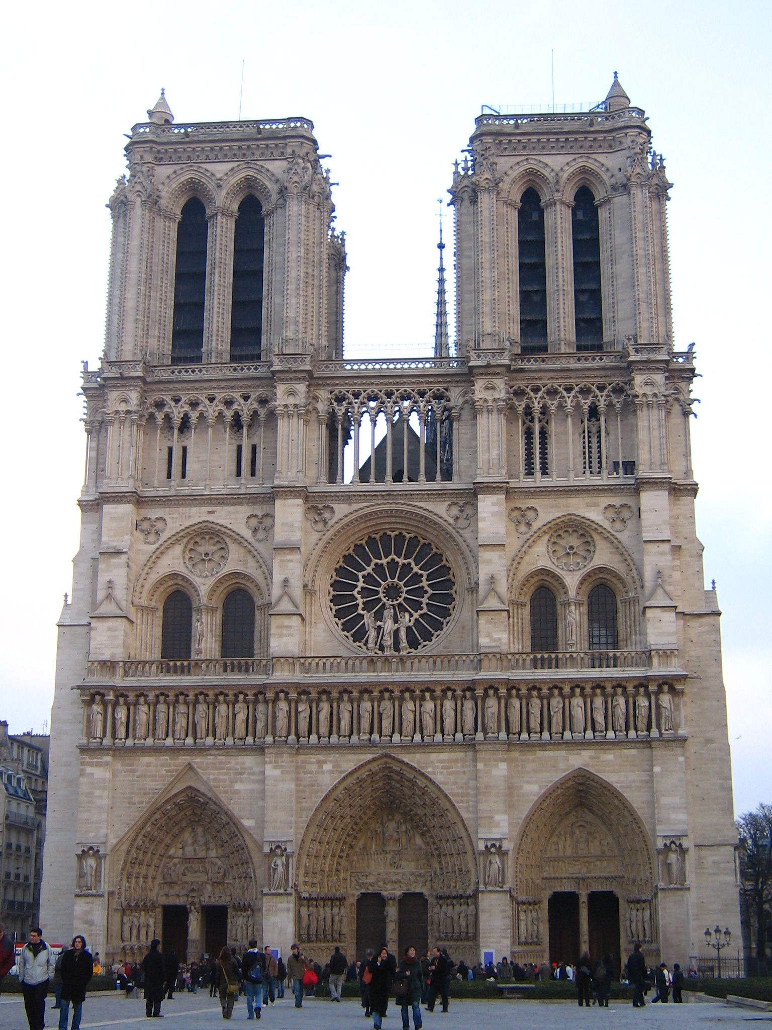
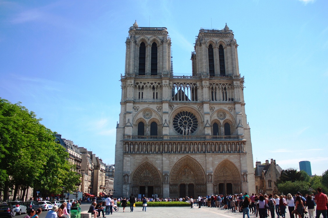
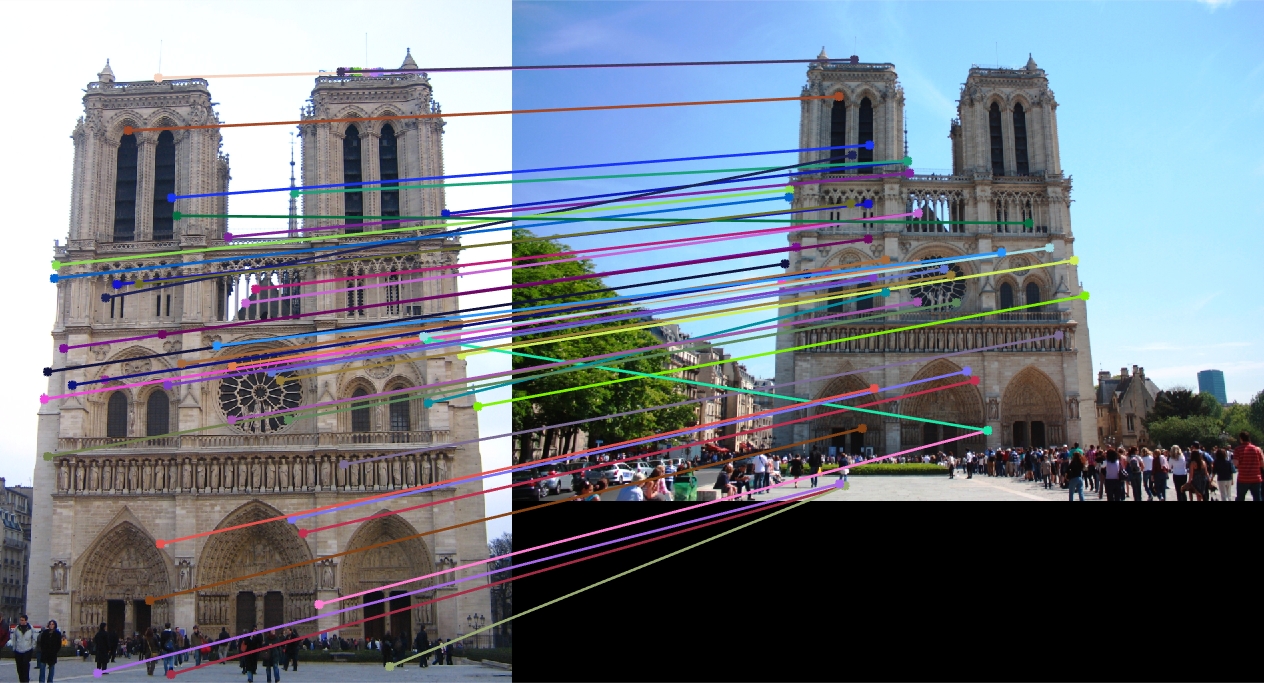
Notre Dame: 1

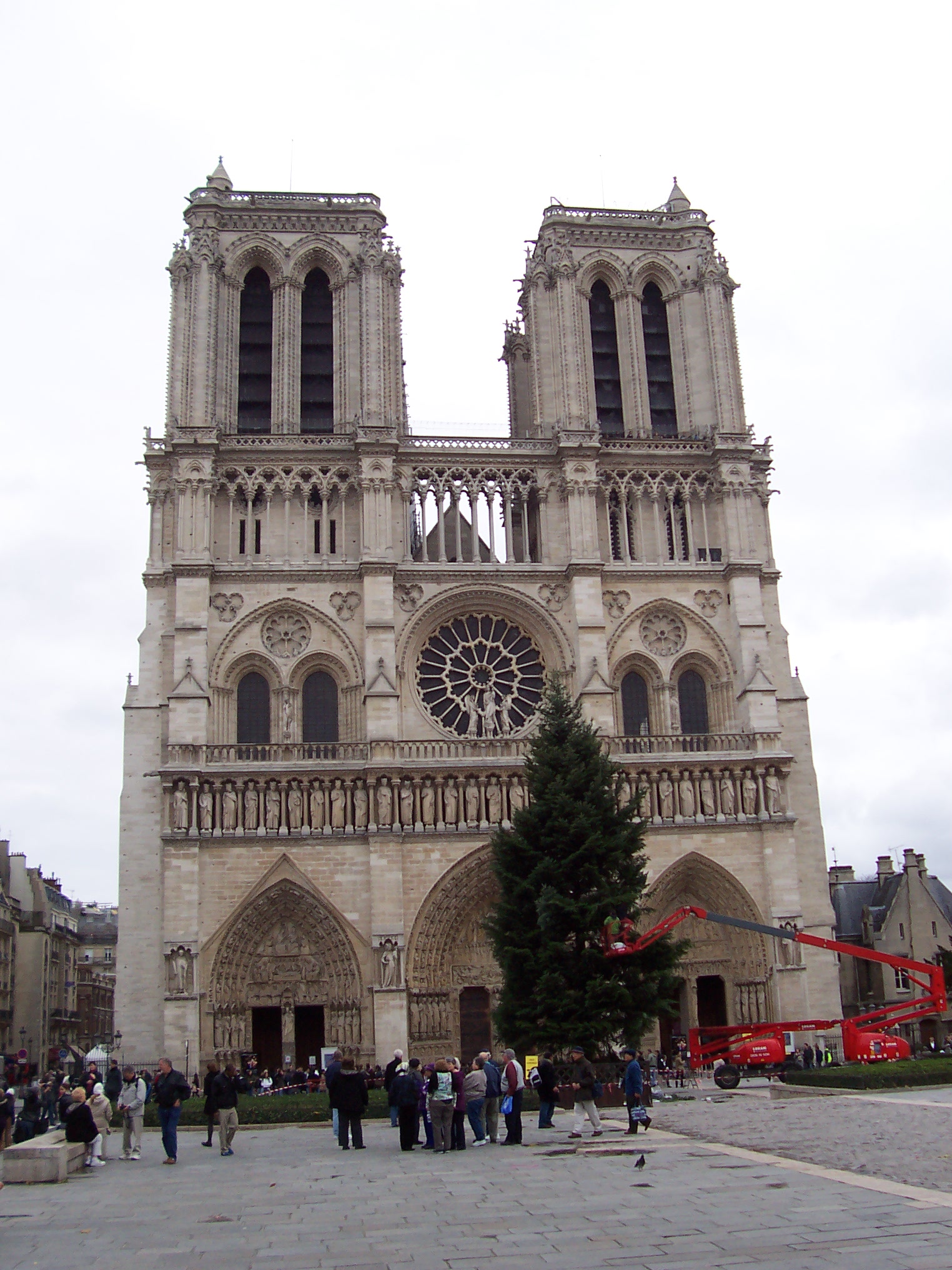
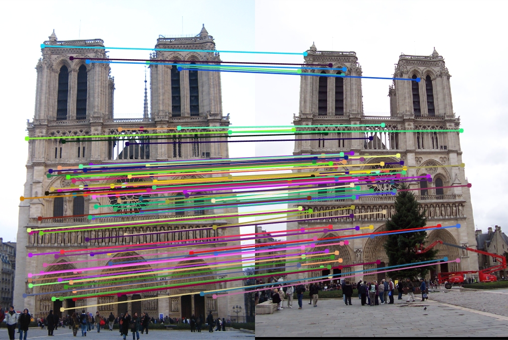
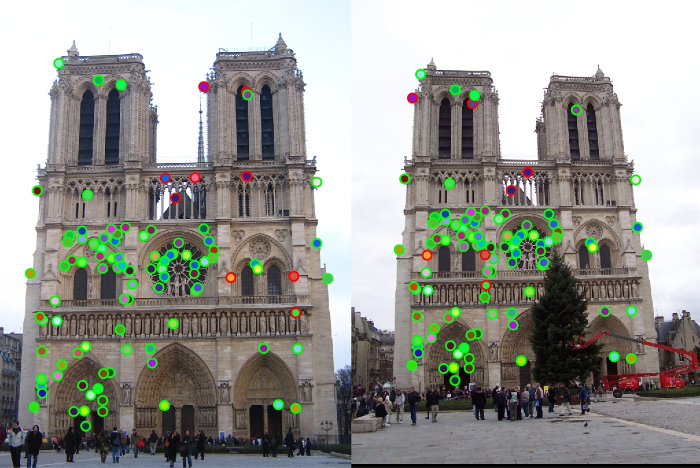
Of the top 100 confident matches, Notre Dame had an accuracy of 91%. Most of the variables were manipulated to improve the quality of Notre Dame, as it was the image used primarily for testing. However, the renormalization concept actually lowered the accuracy of Notre Dame.

Mount Rushmore

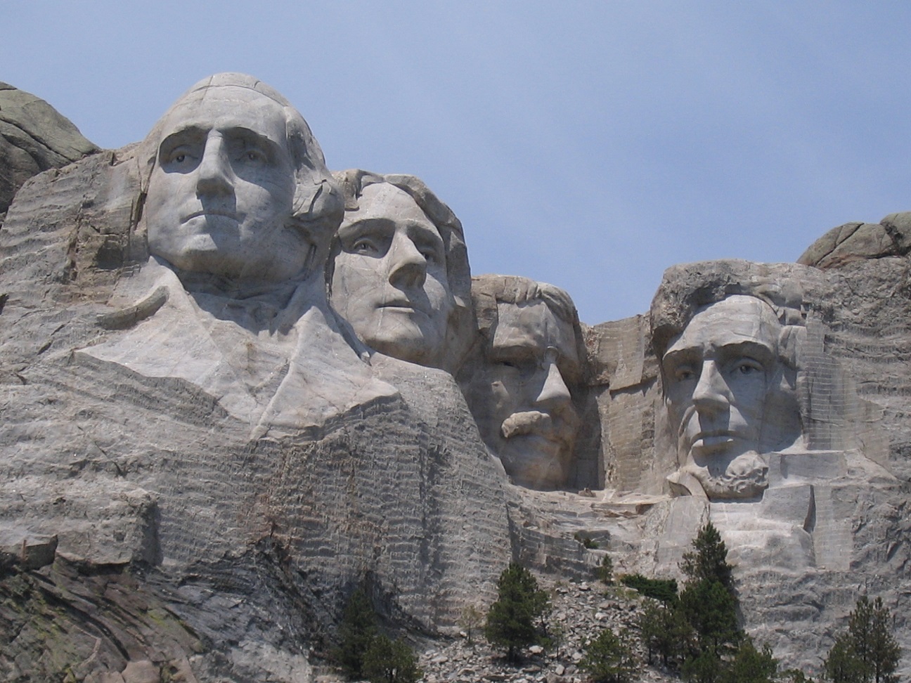
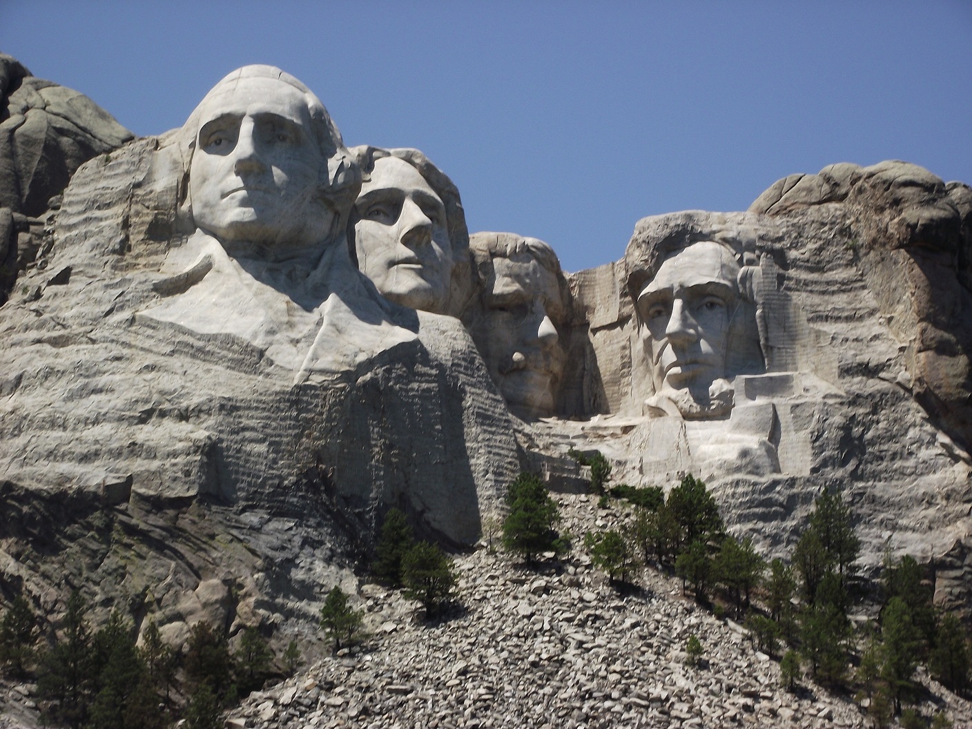
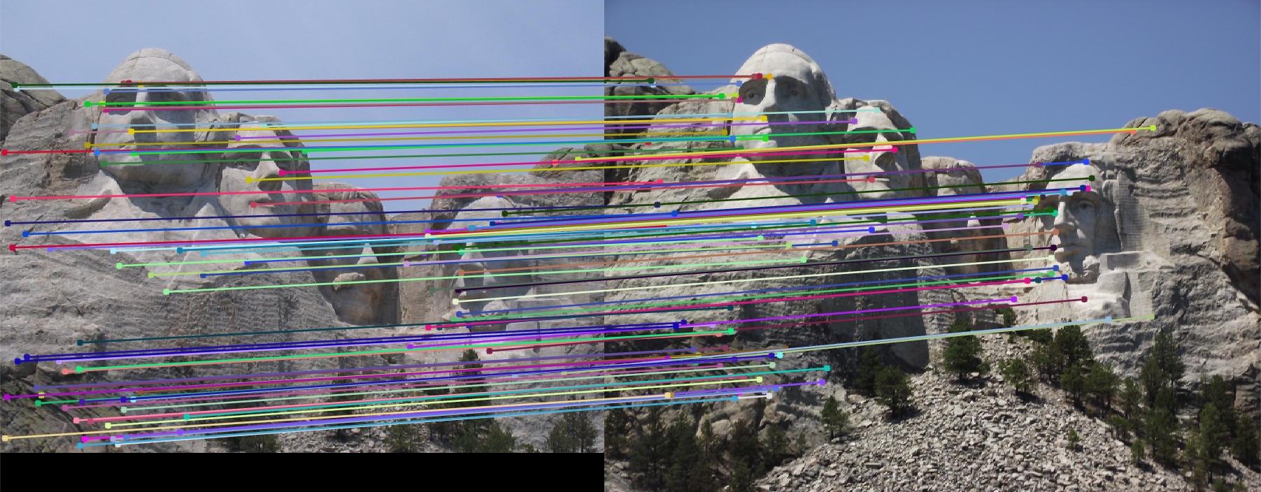
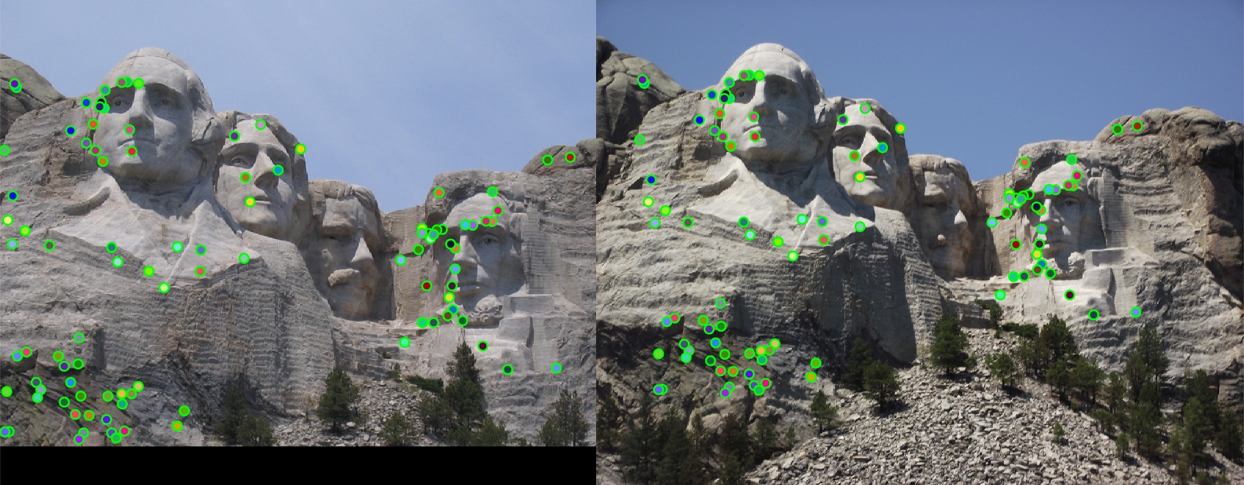
Of the top 100 confident matches, Mount Rushmore had an accuracy of 100%. Before implementing thresholding, Mount Rushmore had a much lower accuracy of roughly 28%, and almost all the points came from the rocks on the bottom.

Episcopal Gaudi

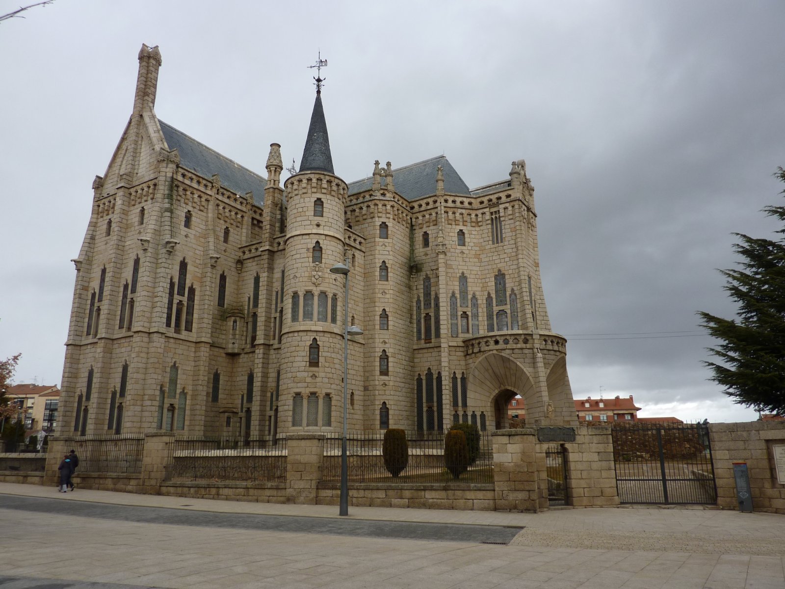
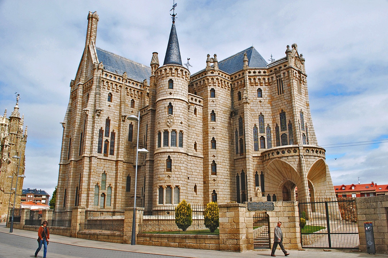
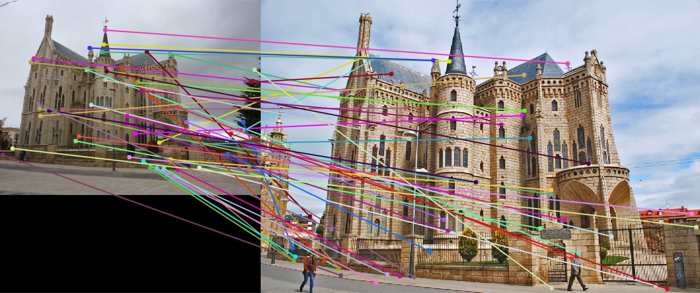
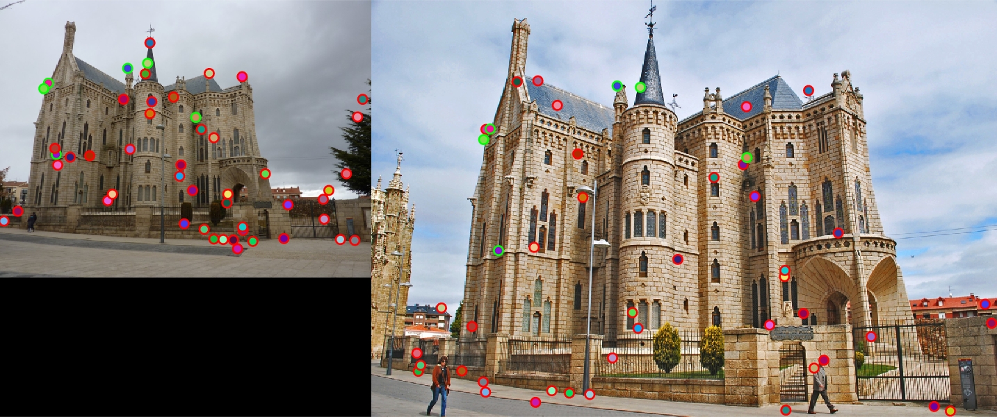
Of the top 40 confident matches, Episcopal Gaudi only had an accuracy of 12%. This is most likely due to the large shift in scale between the two images.

Pantheon

These images no longer have ground truth correspondence, but by looking at the image, it appears as if the image did an overall good job on matching the points. However, the two images were already very similr to each other, so this behavior was intended.

Notre Dame 2

To see things more clearly, only the top 50 confident matches are shown from here on out. Unfortunately, because of the much larger difference in scale, several of the points were matched incorrectly, as scale was not accounted for in the implementation. A lot of points were matched up to a repetition (like a very similar window) as well. However, a good number of the points were still matched up correctly.

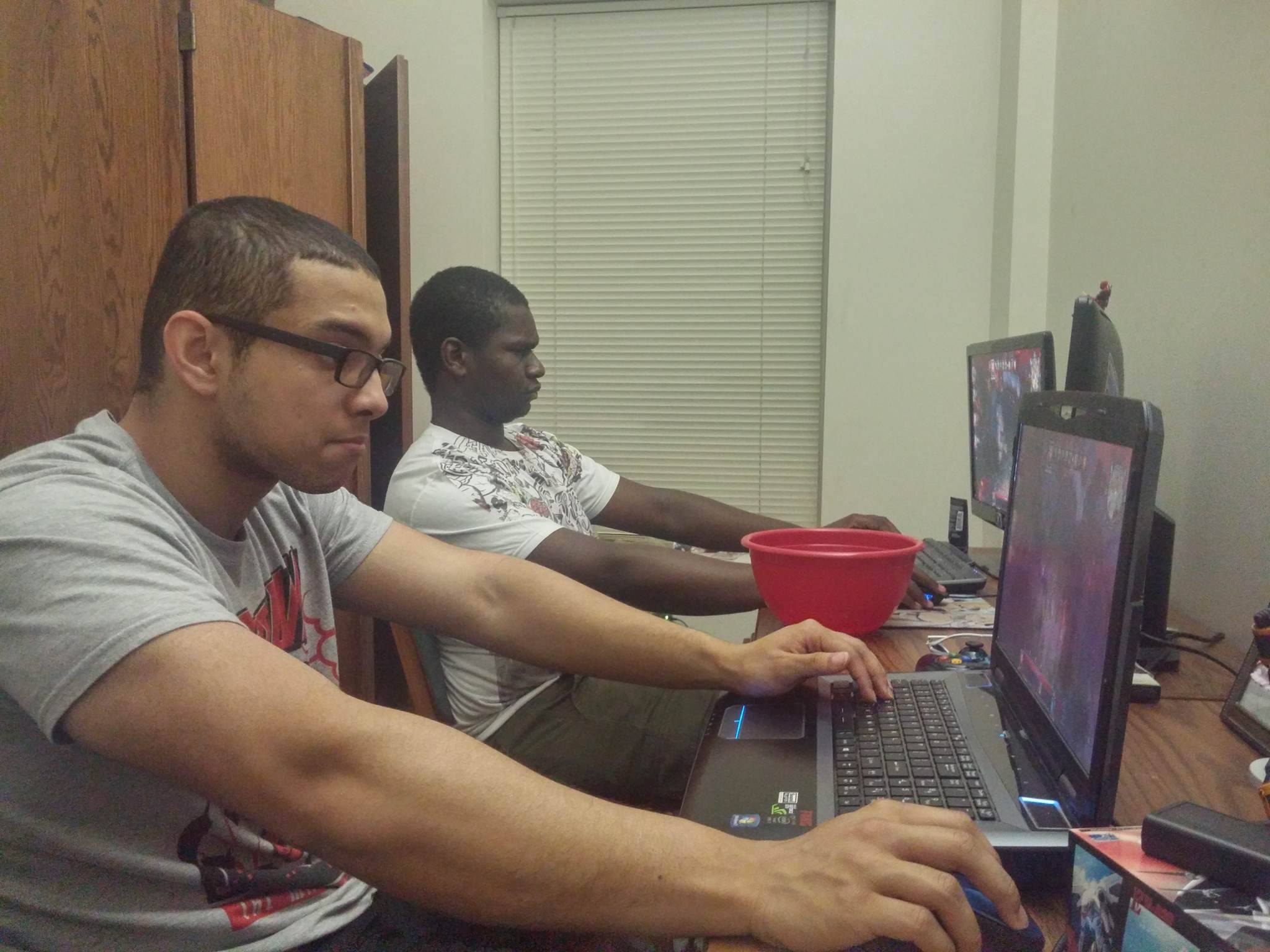
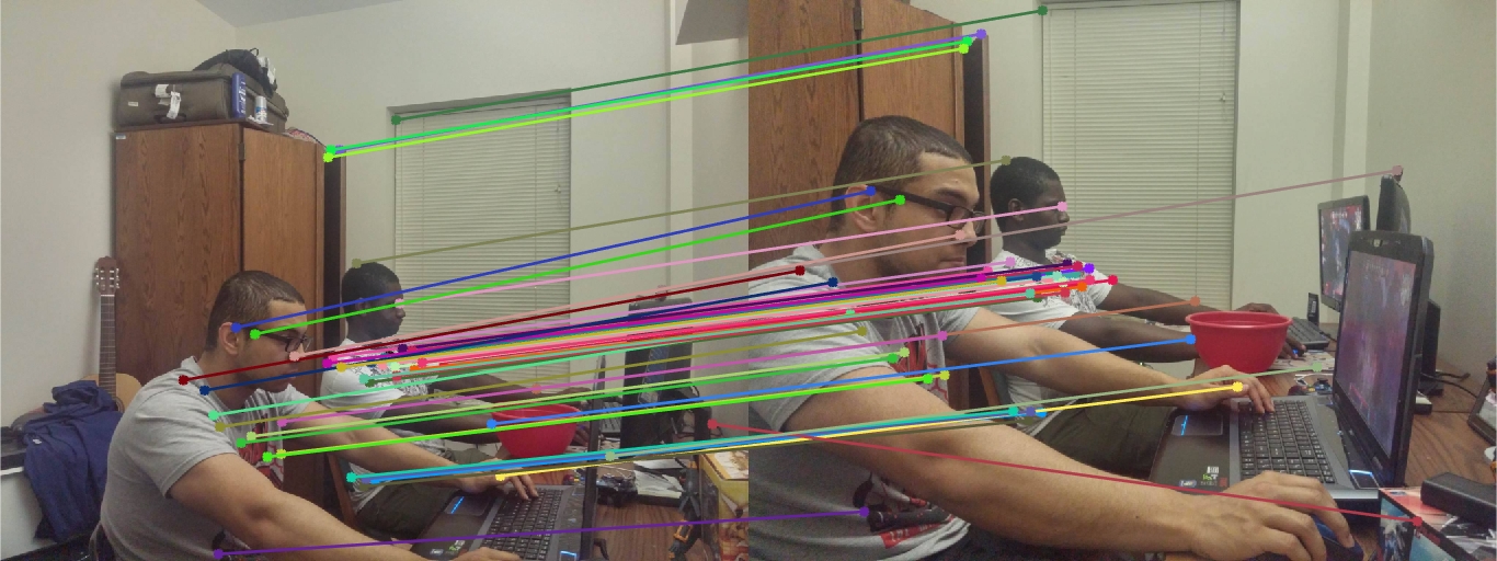
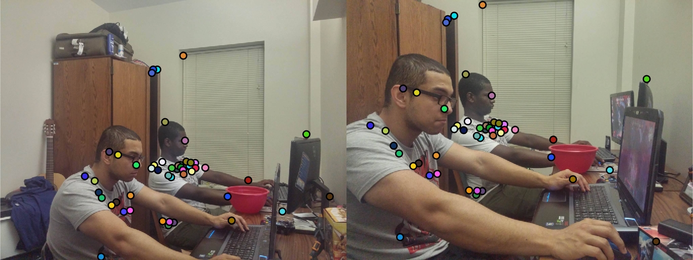
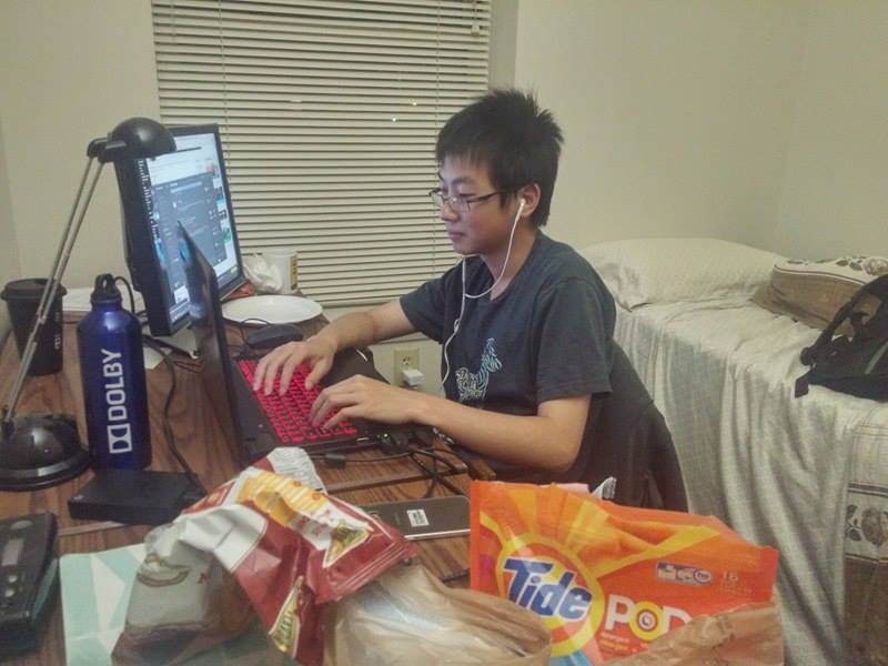
Roommates 1

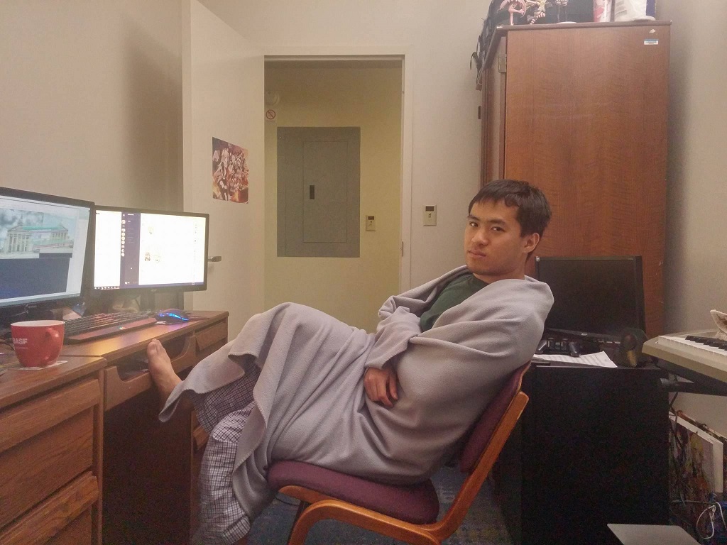
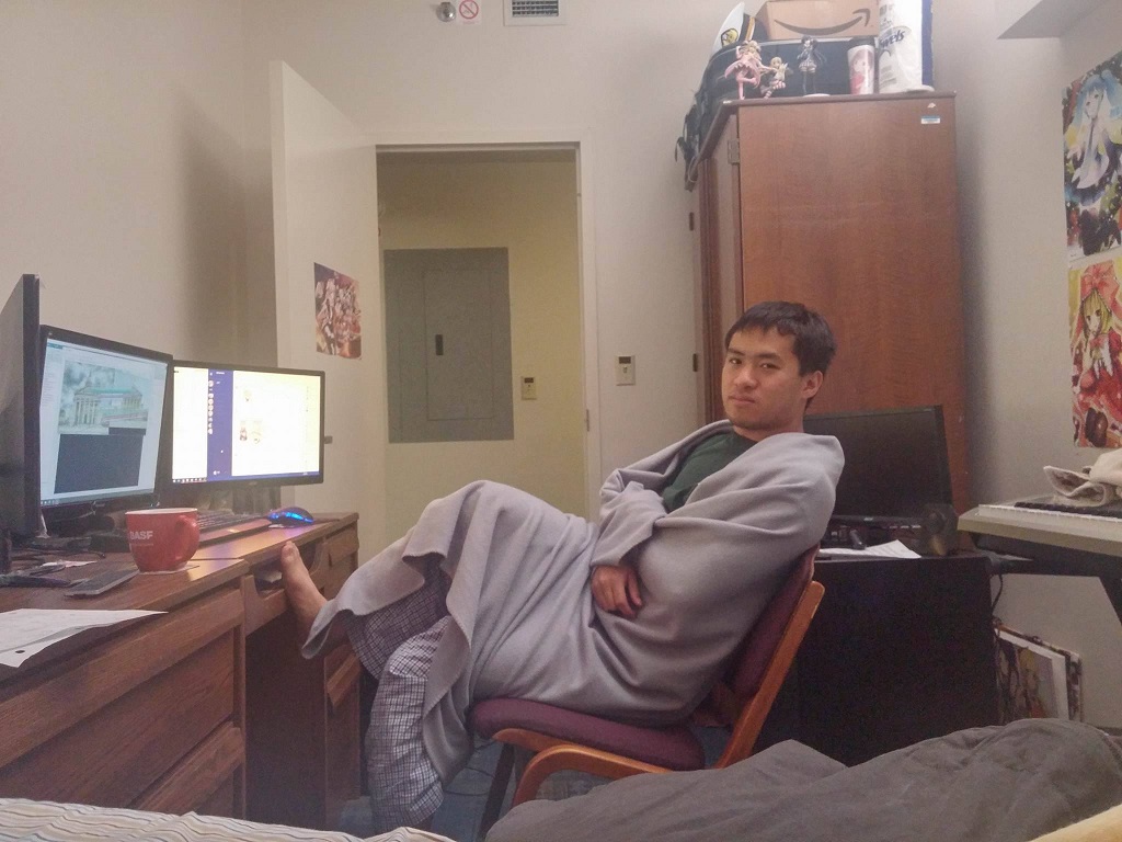
These are some pictures I took of my roommates. Since these two pictures had very little change in them, almost all the points appear to have been identified correctly.

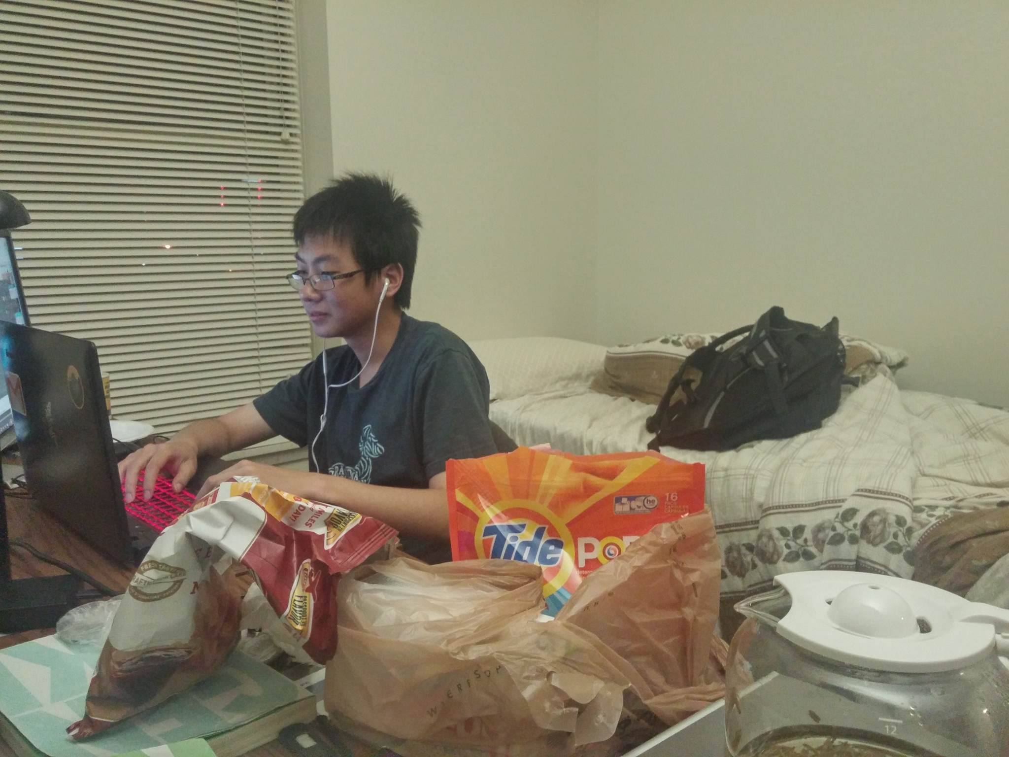
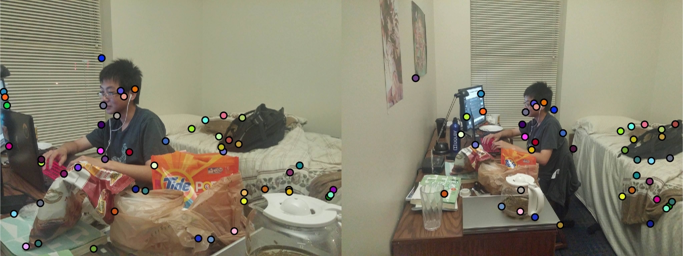
Roommates 2

These are some pictures I took of my roommates. Once again, very little change in the two images, which resulted in most of the points being identified correctly.

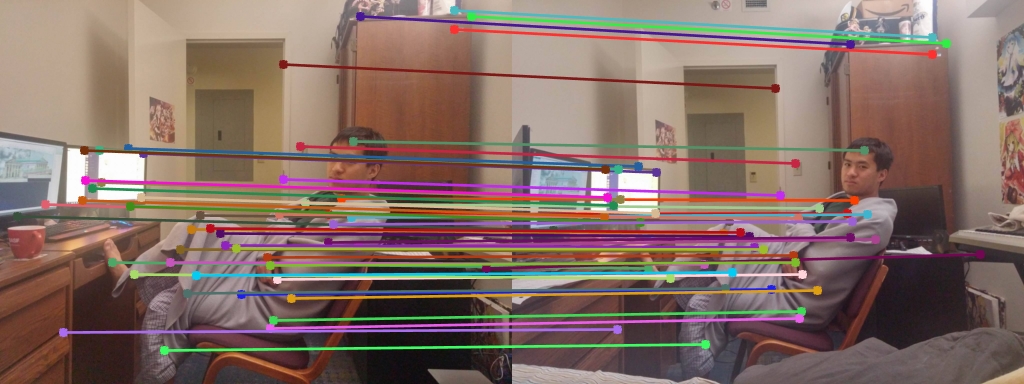
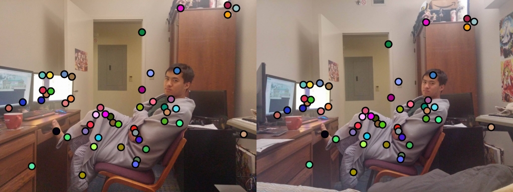
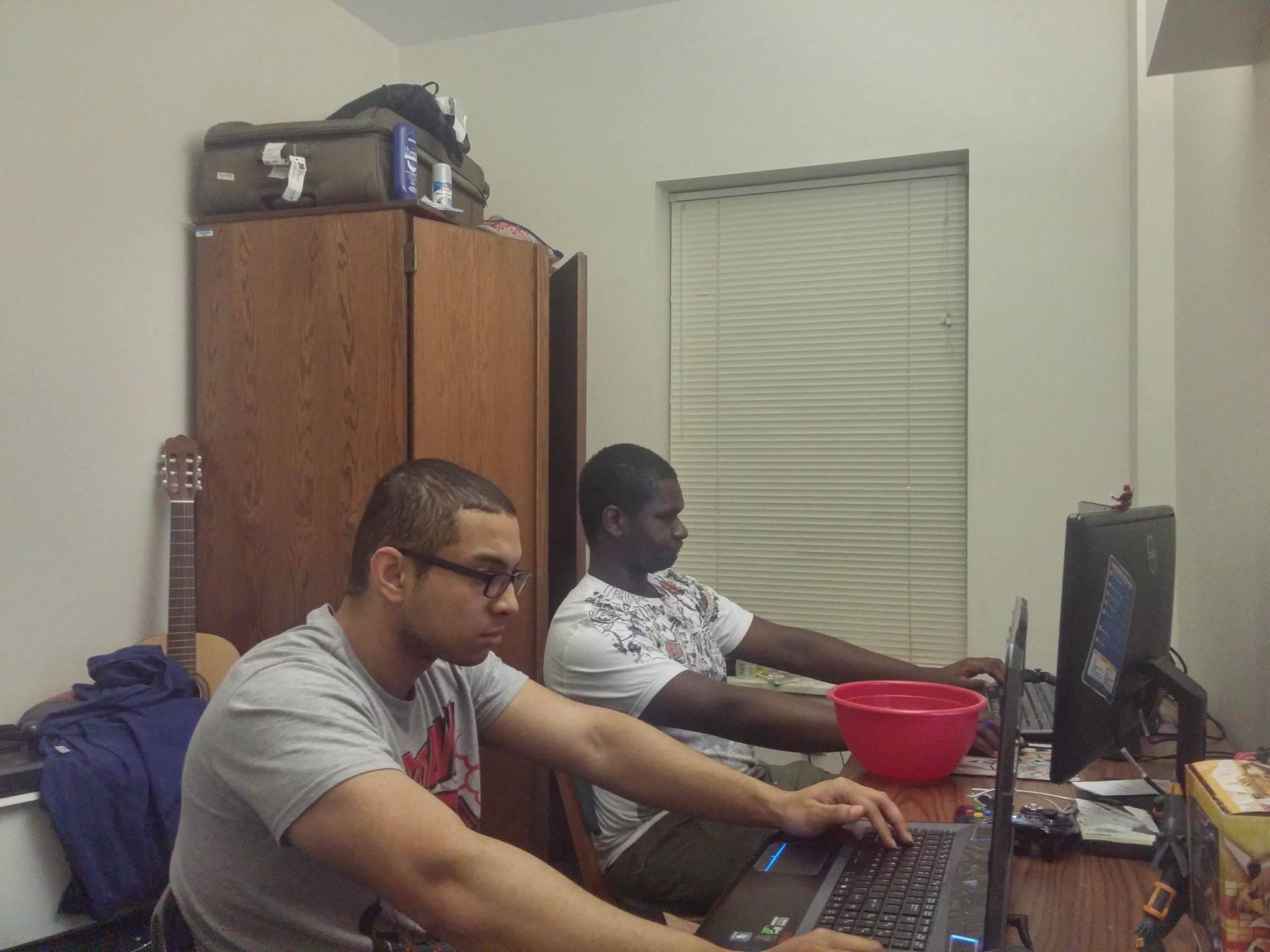
Roommates 3

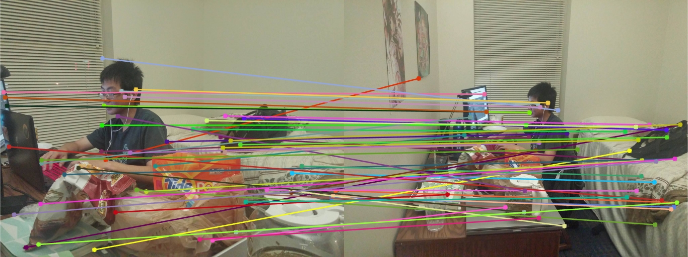
These are some pictures I took of my roommates. This time, very few of the points seem to have been matched correctly, most likely because of the larger change in scale and angle from which the picture was taken from. Some distinct points, such as the edges of the monitor and some parts of the backpack were classified correctly, but most points appear to be all over the place.

3DCG 1

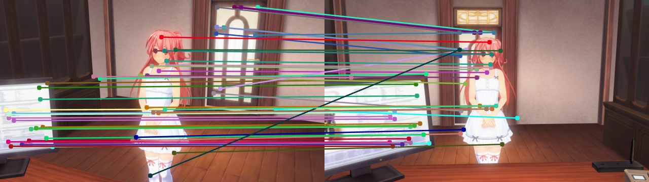
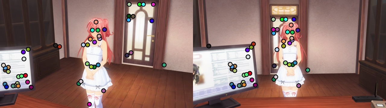
Just for fun, I tried out the algorithm with some 3DCG images from games. Aside from one glaring error (the diagonal line) and a couple of inconsistent points on the door, all the points seem to be pretty accurate. More points seem to be coming from the monitor in the screen however, which may be a sign that my threshold for cornerness may still be too low, as the points there do not seem very distinct.

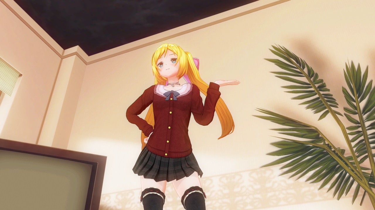
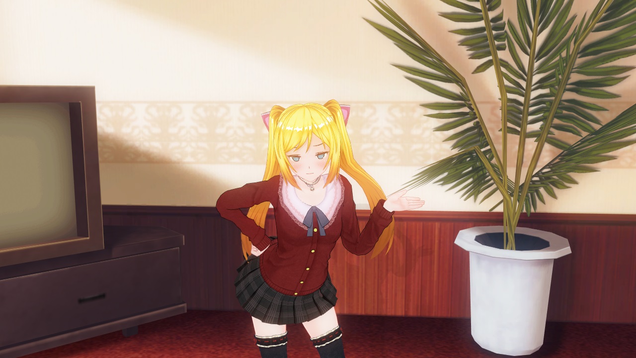
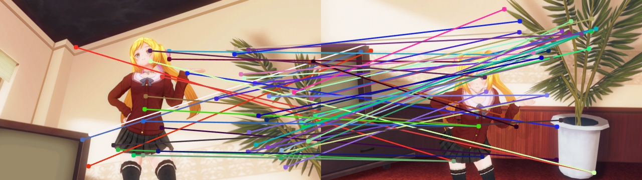
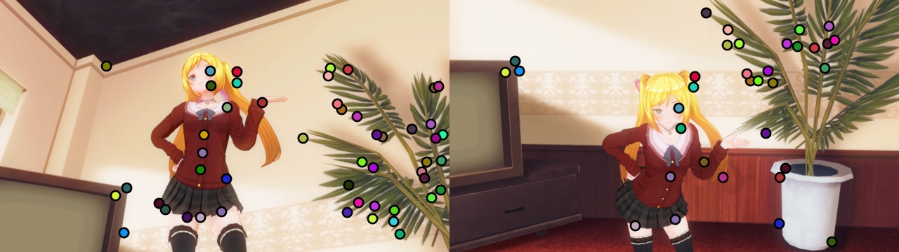
3DCG 2

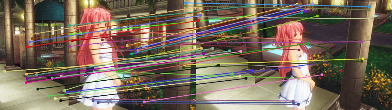
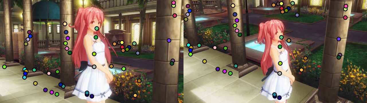
The accuracy of this one was actually quite surprising. There was an angle shift between the two images, but it appears that almost all the points have still been identified correctly between the two images. However, any larger angle shift would likely no longer work, such as the one in Roommate 3.

3DCG 3

Unfortunately, an angle larger than the one shown previously no longer shows many points matching up to each other, which would require more work to the algorithm rather than just implementing the baseline.