Project 2: Local Feature Matching
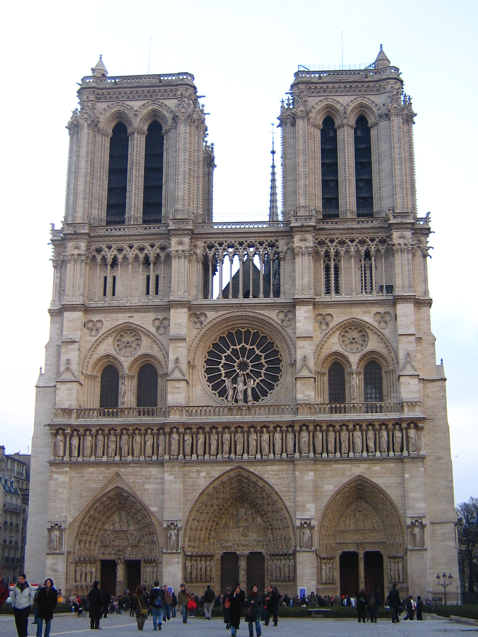
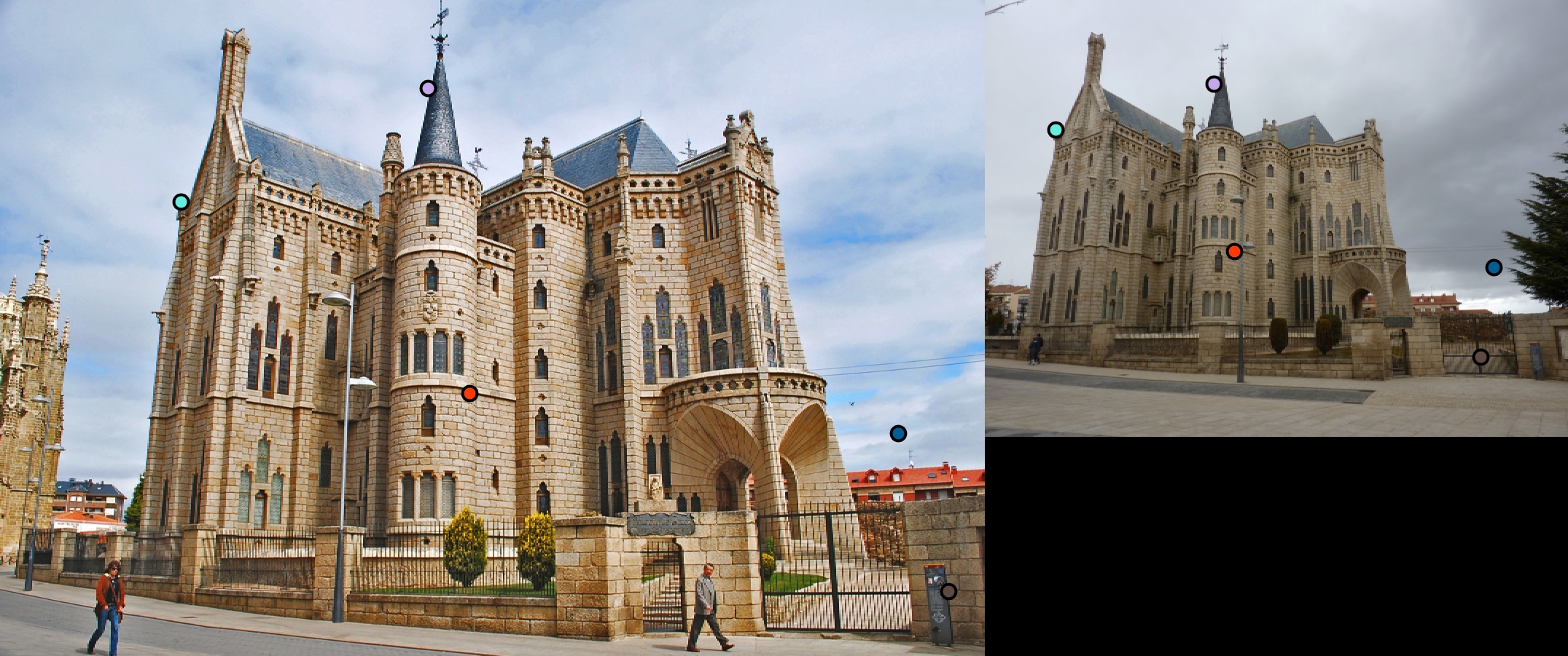
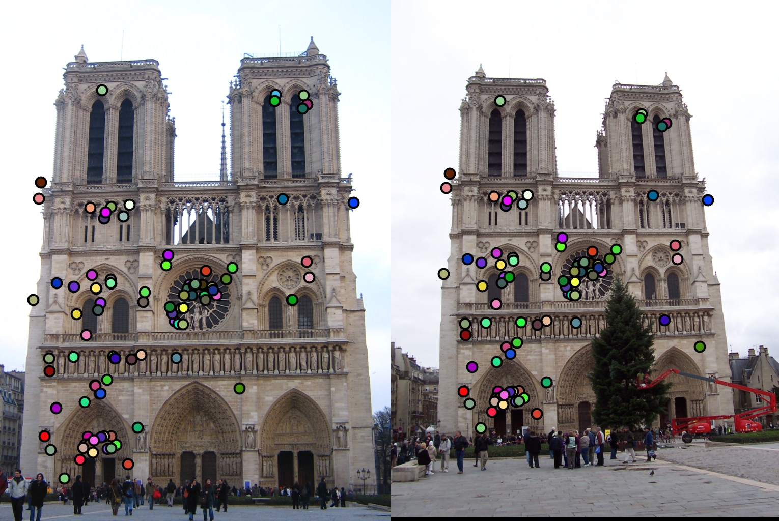
Main image used for testing.
For my project I implemented Matching using pdist2, a radial version of the SIFT like feature described in class, and added adaptive non-maxima suppression to the harris corner algorithm described in class. I will break this write up into 3 sections:
- Final results
- Implementation details
- Analysis of design decisions
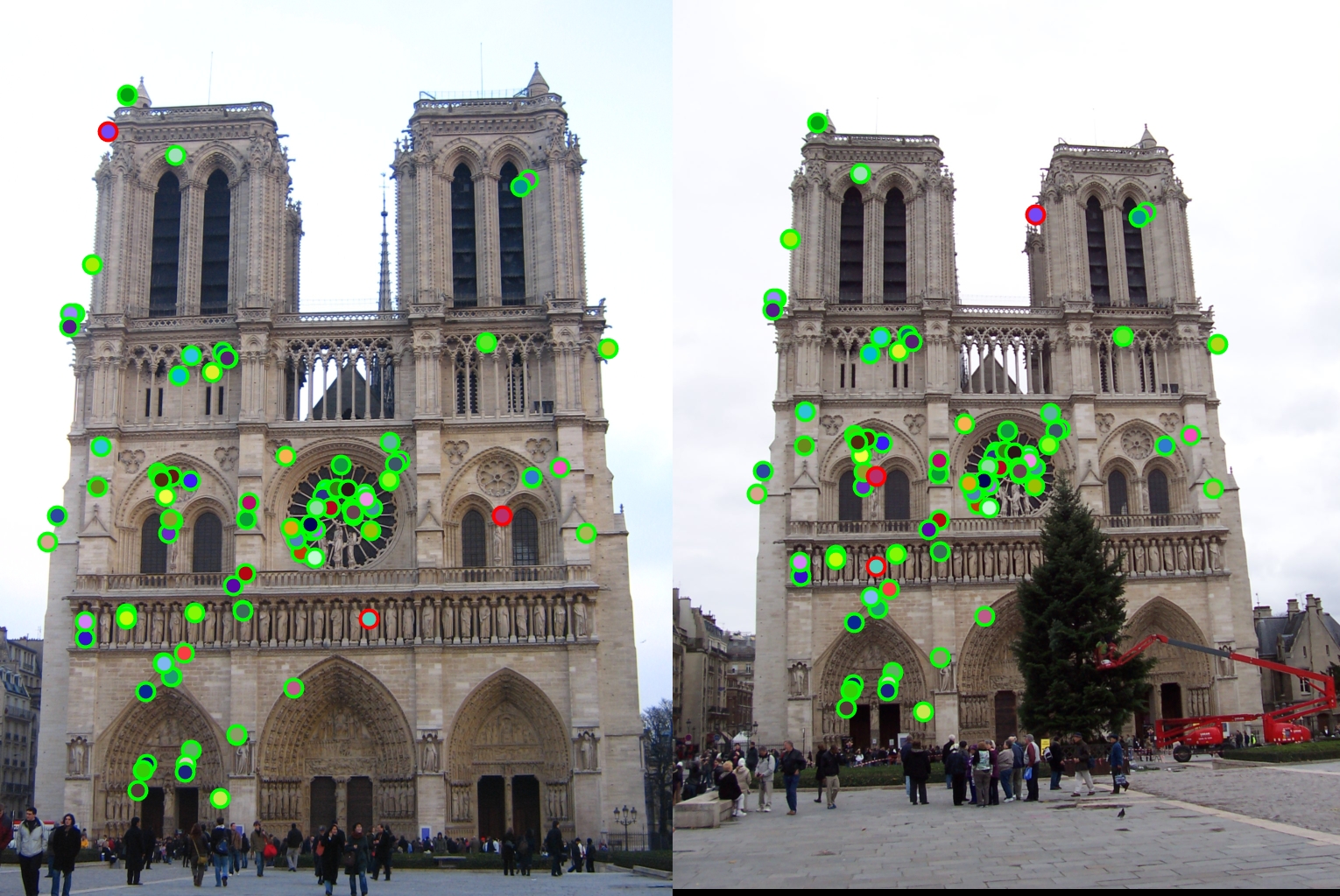
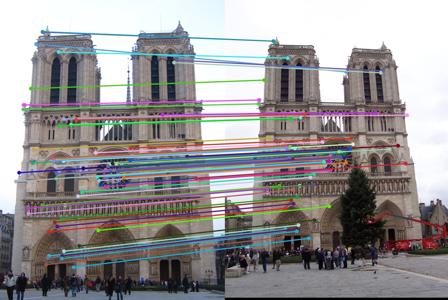
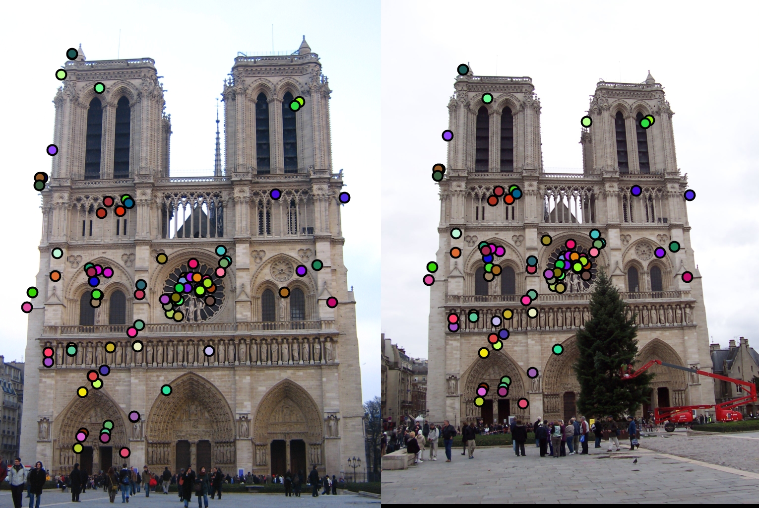
Final results
|
|

|
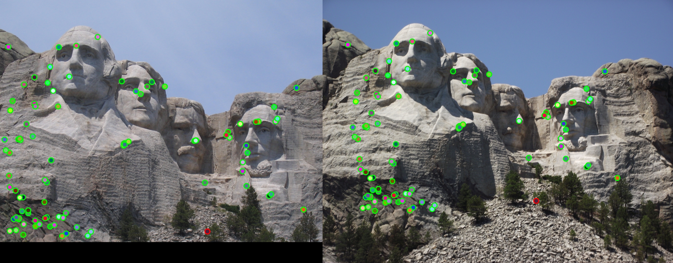
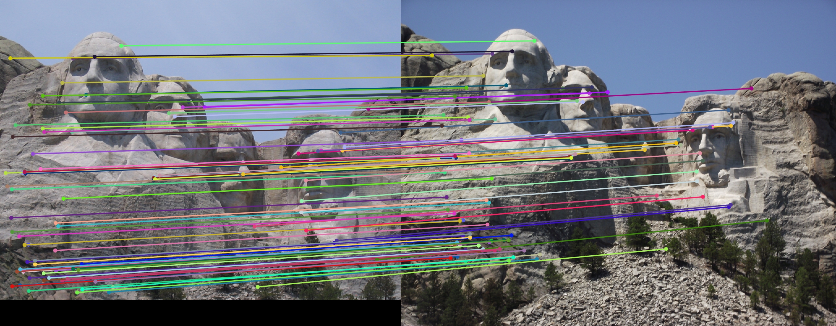
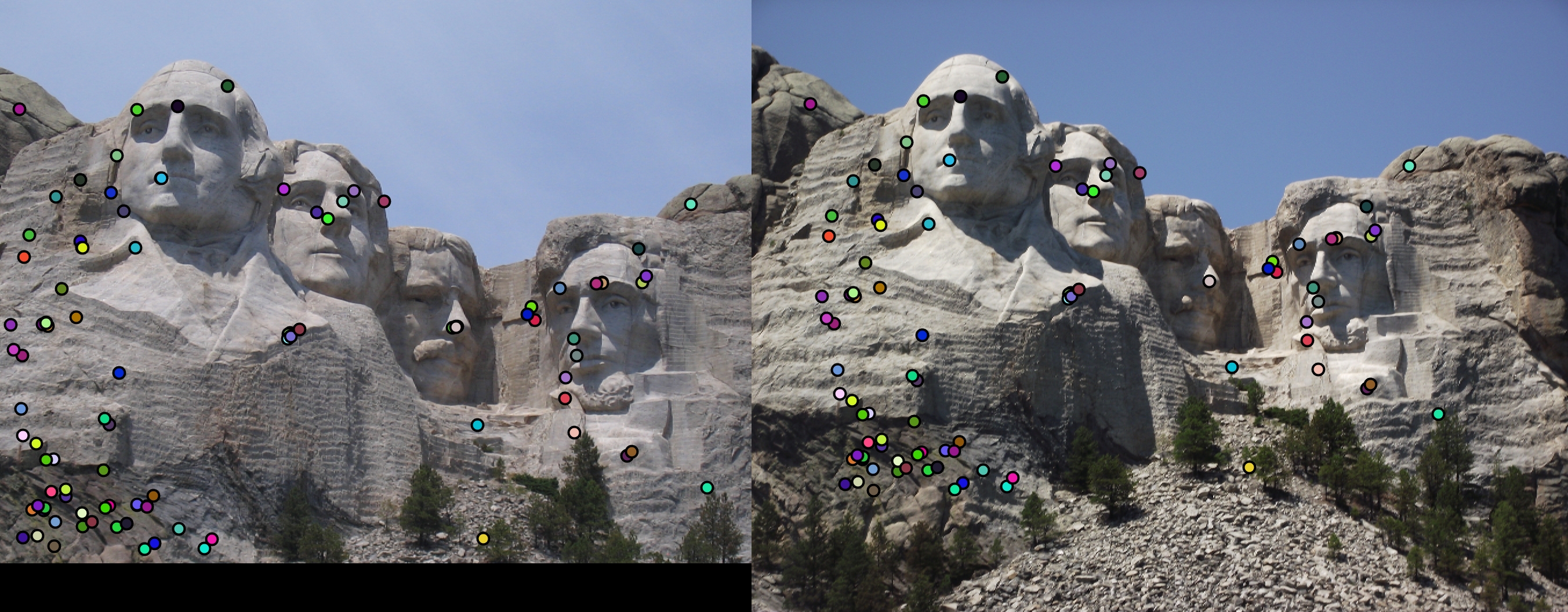
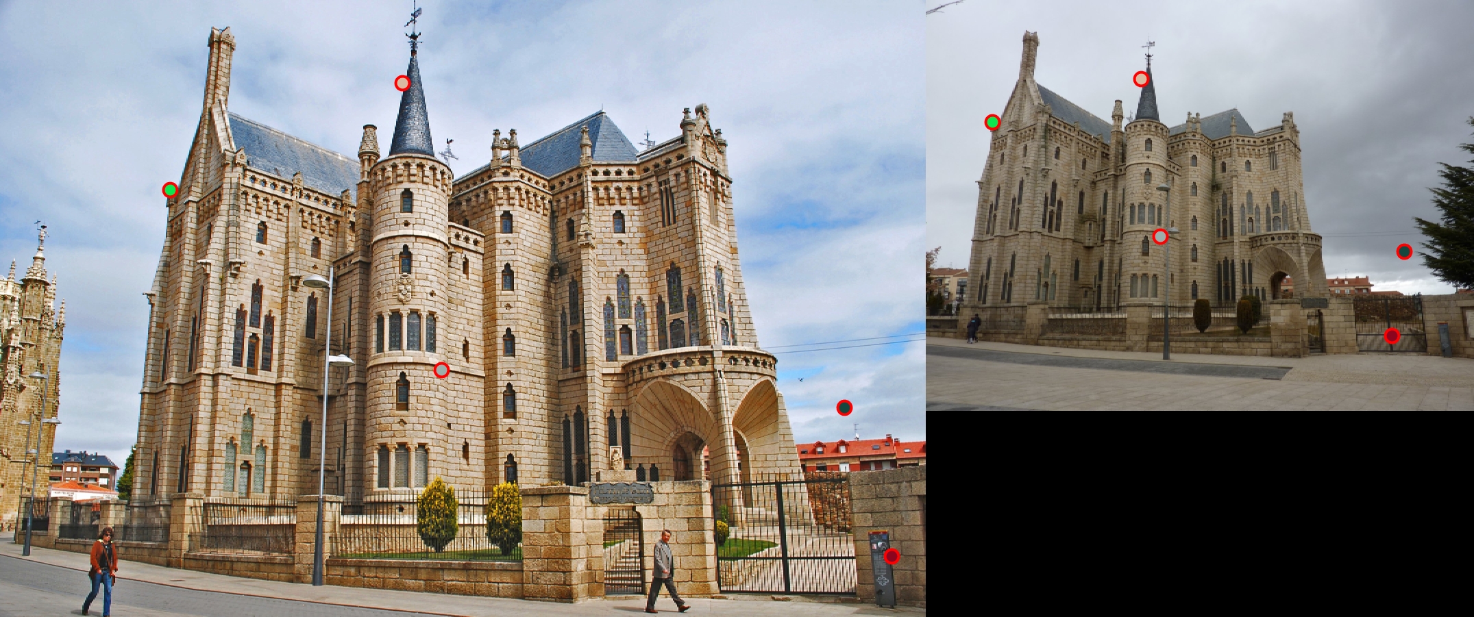
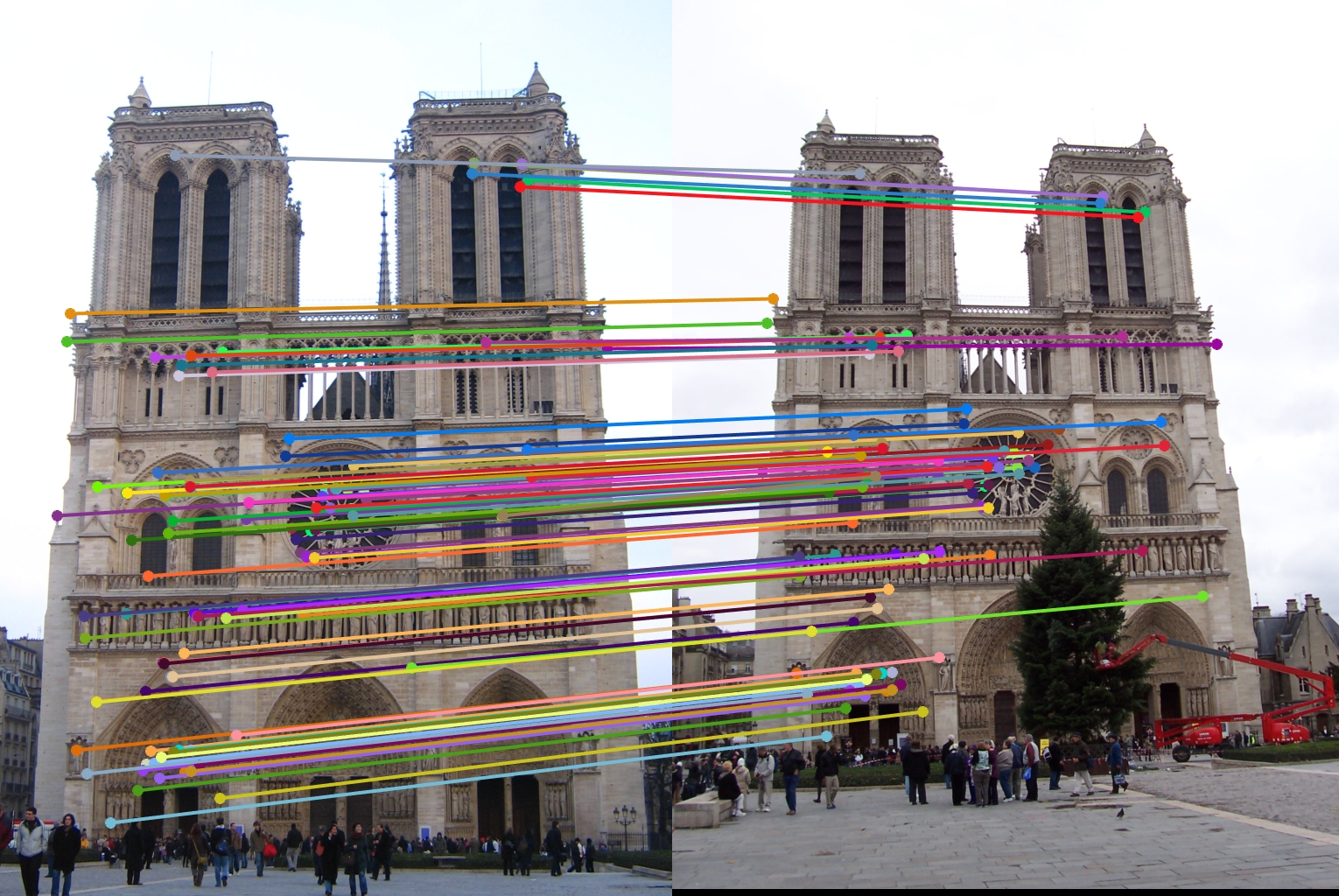
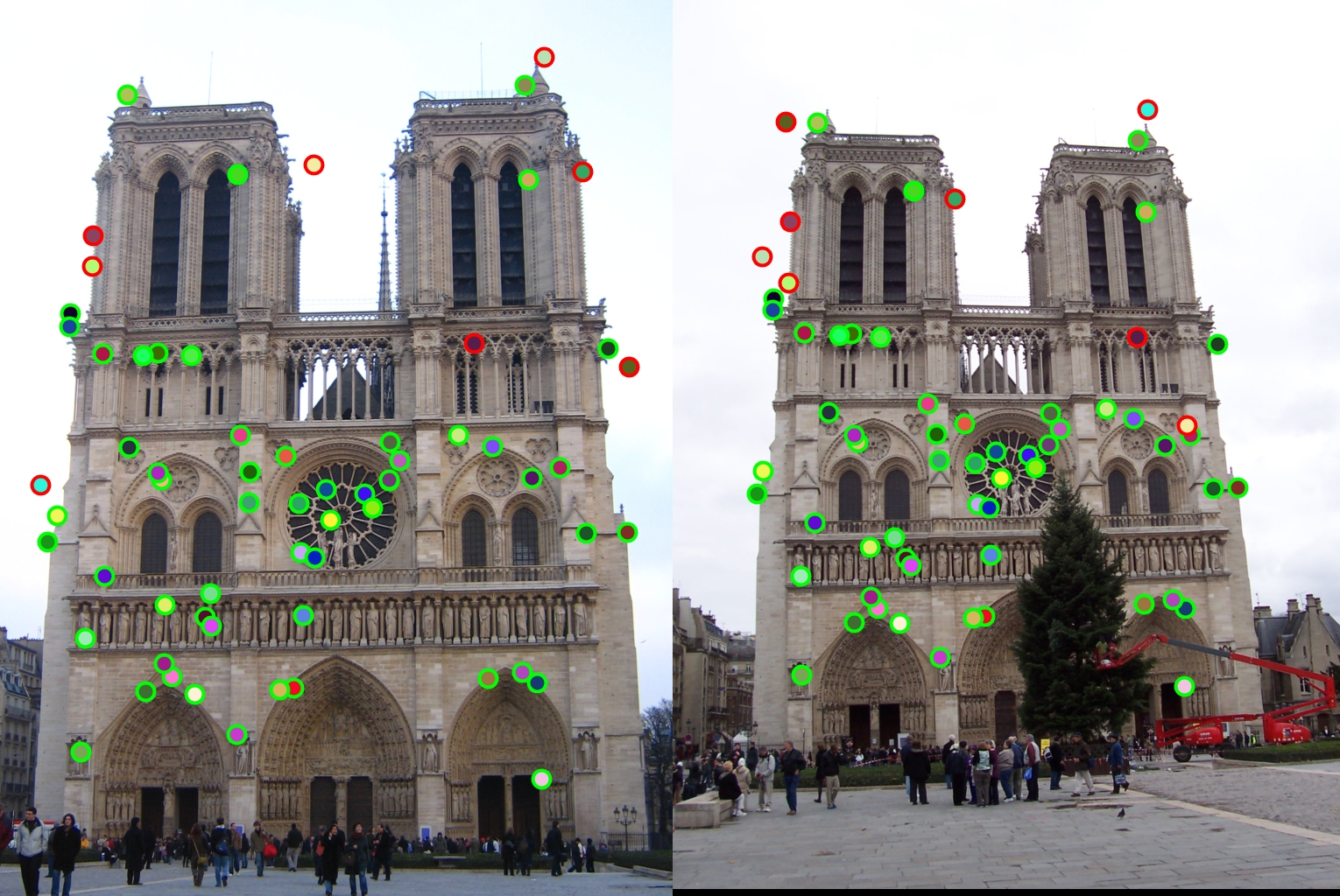
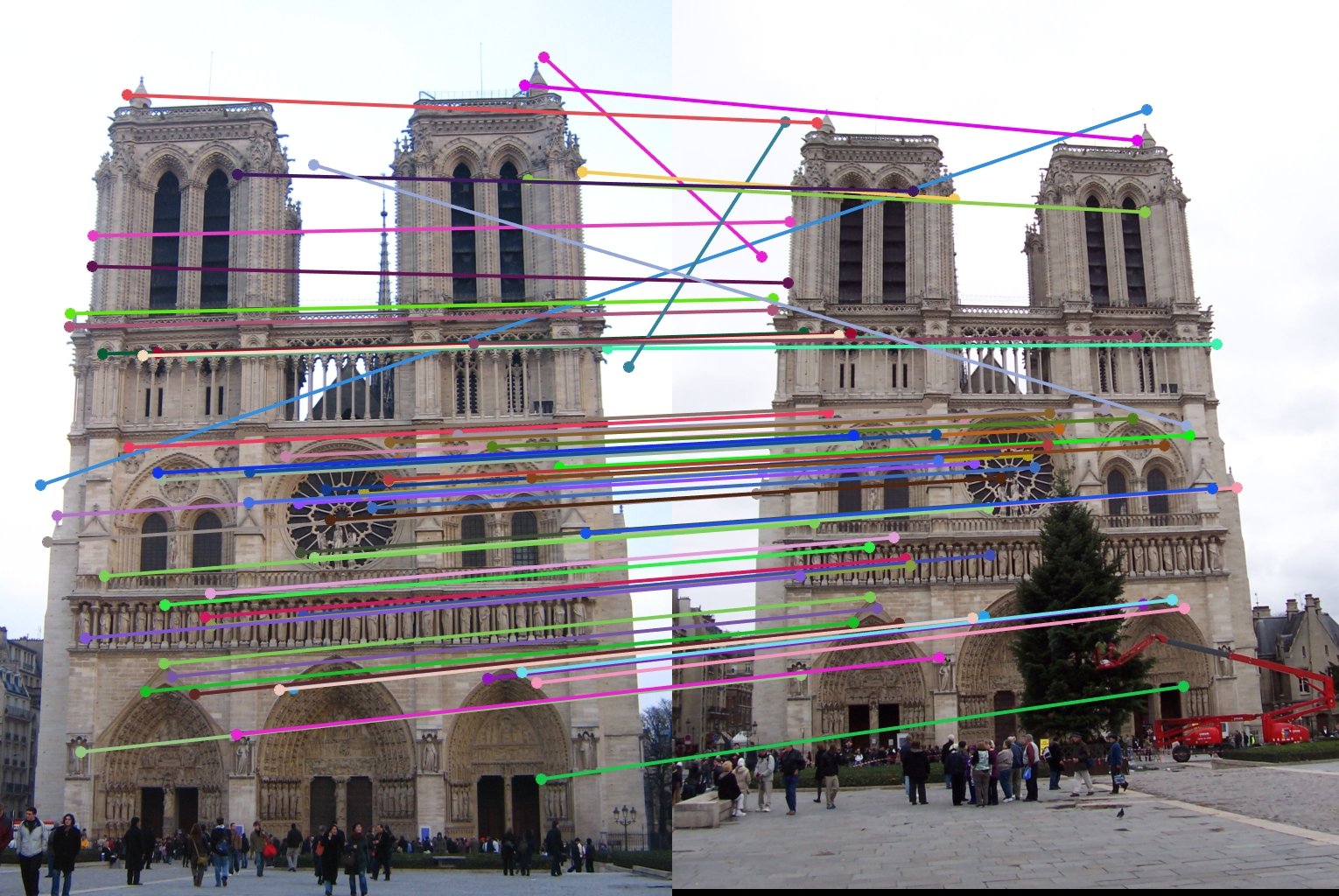
For all image pairs I only took the top 100 matches and had 97% accuracy for Notre Dame and 99% accuracy for Mount Rushmore. However I was only able to make 5 bad matches with the Episcopal Gaudi pair.
Implementation Details
match_features
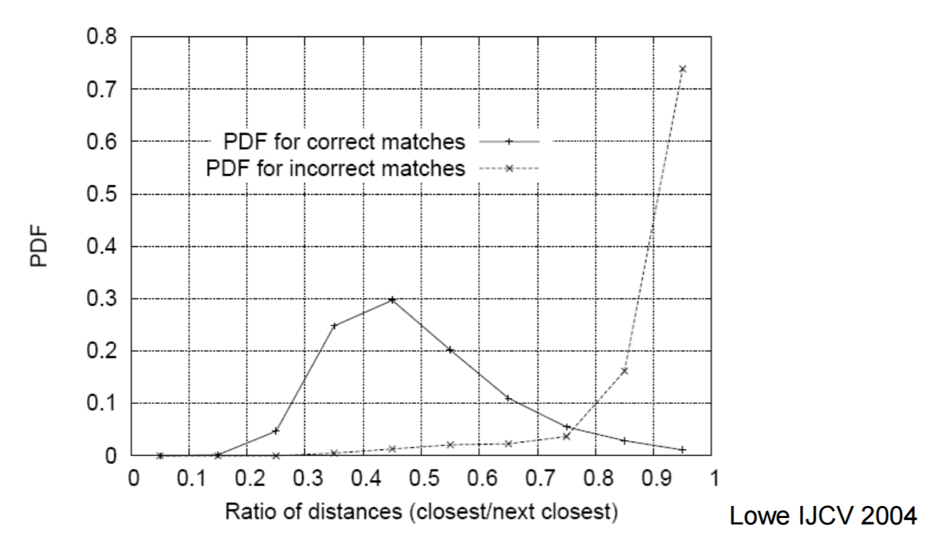
Graph from the lecture 10 slides.
In my implementation I used pdist2 pre-calculate the distance between all the features at once in a matrix. Due to everything being in a matrix, all I had to do to find the nearest neighbor to each feature was to sort each column and get the first index. I then calculated the Nearest Neighbor Distance Ratio to get the confidence for that matching. I also included some filtering to remove NNDRs that we less than .75. I chose this as the limit because in the graph of the PDFs for correct matches the professor showed in class (displayed to the right) the likely hood of a match being incorrect greatly increased after that number. The entirety of my matching code is shown below.
NNDRLimit = .75;
currentMatch = 0;
dist = pdist2(features1, features2);

for f1 = 1 : dim1(1)
    % get eclidean distances for this feature to the others
    dists = dist(f1, :);

    % find top 2 indexes
    [sorted, indexes] = sort(dists);

    % nearest neighbor calculation
    NNDR = sorted(1)/sorted(2);
    % if NNDR is low enough add match
    if(NNDR < NNDRLimit)
        match = [f1, indexes(1)];
        matches(currentMatch + 1,:) = match;
        confidences(currentMatch + 1) = NNDR;
        currentMatch = currentMatch + 1;
    end
end
get_features
When implementing get_features I tried to reduce the amount of operations per feature as much as possible. So, I calculated my the magnitude and direction of each pixel by running imgradient over the whole image. This reduced the per patch calculations to just grabbing the patch for that feature out of the two matrices. This also allowed me to convolve the all of the magnitude with the dampening gaussian at once further reducing the operations per feature. Because of these optimizations the only per-pixal calculations I had to do was the binning for the actual feature creation. The code for this is shown below.
% place magnitudes in bins according to its angle and patch coordinates
for row = 1 : feature_width
    for col = 1 : feature_width
        [theta,r] = cart2pol(col - 7, row - 7);
        theta = rad2deg(theta);
        if r <= 6
            circle = 1;
        else
            circle = 2;
        end
        bin1 = getBin(theta);
        bin2 = getBin(angles(row, col));
        feature(circle, bin1, bin2) = feature(circle, bin1, bin2) + mags(row,col);
    end
end
The getBin call simply maps the given angle to one of the 8 quadrants ranging from -180 degrees to 180 degrees using if statements. Instead of implementing the standard SIFT 4x4 grid of histograms I implemented a radial approach designed after GLOH. Unlike GLOH however I decided to only have two circles, one of radius 6 and one of radius 12. I did this because the size of the feature was only 16x16, so the furthest polar radius any cell could be was ~11 making the radius 15 circle a wast of memory.
get_interest_points
One of the main things I did in my corner detector to improve the response rate was to use a binary image instead of a grey scaled one. The code I used to do that is below. As shown below I also blur the final binary image with a gaussian before getting the gradients. In my testing using a 6x6 gaussian filter with a sigma of 1 seemed to produce corners with the highest response.
% convert the image to binary
grayscaled = mat2gray(image);
bin =  imbinarize(grayscaled, 'adaptive');
blurred = imfilter(bin, fspecial('gauss', 6, 1));
[Ix, Iy] = imgradientxy(blurred);
In my corner detector instead of doing regular non-maxima suppression I implemented adaptive non-maxima suppression. I did this by using colfilt to find the maximums for all 6x6 neighborhoods in the image. I then only accepted corners that were 10% bigger than the surrounding pixels.
% get harris corners
har = gIx2.*gIy2 - gIxy.^2 - alpha * (gIx2 + gIy2).^2;
% find neighbrhood max
harmax = colfilt(har,[6 6],'sliding', @maxNeighbors);
% remove values that aren't atleast 10% bigger than their neighbors
nonmaxima = (har>harmax*.9)&(har>5);
...
function y = maxNeighbors(x)
    x = max(x);
    y = x;
end
I also used find() to get the indexes of all the corners. I used to both create the x and y vectors, but to also remove any corners near the edges of the image. that was done to make get_features easier as it no longer had to worry about array bounds when grabbing patches.
Analysis of design decisions
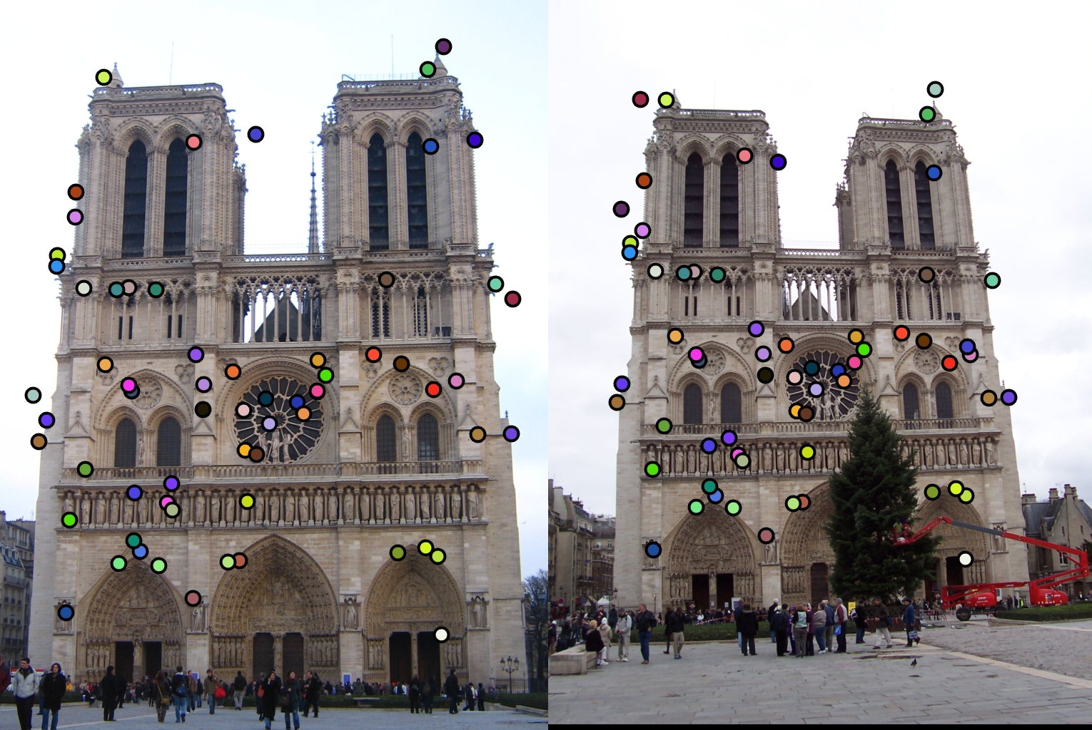
The first design decision I will examine is the switch from the SIFT 4x4 grid to the GLOH like radial approach. The comparison of these two methods is shown below with my final radial approach being the one on top.
|
|
|
As stated before my radial feature was able to get over a hundred matches with the top 100 being 97% accurate. However, while the 4x4 SIFT feature was able to get 100 matches, it only got 94% accuracy. Therefore my radial feature was an improvement.
The second design decision I will examine is the switch from the regular non-maxima suppression to the adaptive one. The comparison of these two methods is shown below with my final adaptive approach being the one on top.
|
|
|
As stated before my adaptive approach was able to get over a hundred matches with the top 100 being 97% accurate. However, the regular approach I implemented only got 64 matches and only 88% accuracy. Therefore my adaptive approach had a significant improvement.