Project 2: Local Feature Matching

Local Feature Description (get_features.m)

            features = zeros(0, 128);

            pad = feature_width/2;
            padimage = padarray(image, [pad pad]);

            [height, width] = size(padimage);
            [grad_mag, grad_dir] = imgradient(padimage);

            x = x + pad;
            y = y + pad;

            for row = 1:length(x)
                tlr_grid = y(row) - feature_width/2;
                tlc_grid = x(row) - feature_width/2;
                
                % colon operator with decimals does not do the same thing as
                %   rounding the decimals.  Rounding reduced accuracy for me.
                warning('off','all')
                patch_mag = grad_mag(tlr_grid:(tlr_grid + feature_width - 1), ...
                                     tlc_grid:(tlc_grid + feature_width - 1));
                patch_dir = grad_dir(tlr_grid:(tlr_grid + feature_width - 1), ...
                                     tlc_grid:(tlc_grid + feature_width - 1));
                warning('on','all')

                patch_mag = imgaussfilt(patch_mag);
                cell_size = feature_width/4;
                
                descriptor = zeros(0);
                for cell_row = 1:4
                    for cell_col = 1:4
                        
                        % Individual cell
                        cc_row = cell_size * cell_row - 3;
                        cc_col = cell_size * cell_col - 3;
                        cell_mag = patch_mag(cc_row:(cc_row + cell_size - 1), ...
                                           cc_col:(cc_col + cell_size - 1));
                        cell_dir = patch_dir(cc_row:(cc_row + cell_size - 1), ...
                                           cc_col:(cc_col + cell_size - 1));
                        
                        d = zeros(1, 8);
                        
                        % Only adding to one bin
                        cell_dir = fix(mod(cell_dir + (180 + 22.5), 360) / 45 + 1);
                        for i = 1:cell_size^2
                            bin = cell_dir(i);
                            d(bin) = d(bin) + cell_mag(i);
                        end
                        [descriptor] = [descriptor d];
                    end
                end
                
                features(row, :) = descriptor ./ sum(descriptor);
            end
        

Once we get interest points, we compute a feature descriptor from each point by looking at the surrounding pixels of the interest point. We do this by creating a window over each pixel and calculating the gradient magnitude and orientation of each pixel. From there we categorize the orientation into one of 8 orientations (histogram) and add the magnitude to that orientation bin. For each interest point we calculate a 4x4 grid of 8 orientations (16 histograms of size 8 domain) and we get a 126 dimension feature descriptor. The code is long, but this is how I may have done it with another programming language. I thought the calculation of the bin instead of using if-statements was cool though. I also run a gaussian on the window because closer pixels matter more to a center pixel than further ones.

Histogram Orientation Interpolation (match_features.m)

            % Sharing to two bins using cosine
            cell_dir = fix(cell_dir + 180);
            for i = 1:cell_size^2
                bin_one = fix(cell_dir(i) / 45) + 1;
                bin_two = fix(mod(cell_dir(i) + 45, 360) / 45) + 1;
                
                r = mod(cell_dir(i), 45) * 2;
                
                d(bin_one) = d(bin_one) + cosd(r) * cell_mag(i);
                d(bin_two) = d(bin_two) + sind(r) * cell_mag(i);
            end
        

For adding to the bins, I decided to perform an interpolation such that a gradient measurement contributes to two different bins. For a gradient vector, it either lies in between two orientations or is that orientation. I find the two orientations (x and x+1) and calculate cosine/sin values of the magnitude and apply those values to the respective orientation histograms. This makes it better for gradient vectors which evenly contribute to two orientations but only gets applied to one. This simple technique increased the accuracies of the ground truth correspondence images (notre_dame 81 - 93, mount rushmore 33 - 39, episcopal_gaudi 6 - 8).

Local Feature Description (match_features.m)

            matches = zeros(0, 2);
            confidences = zeros(0, 1);

            %% Finding closest and second closest neighbors.
            for f1 = 1:size(features1, 1)
                goldDist = realmax;
                goldIndex = -1;
                silverDist = realmax;
                
                % Calculate euclidean distance
                for f2 = 1:size(features2, 1)
                    dist = norm(features1(f1,:) - features2(f2,:));
                    if dist < goldDist
                        silverDist = goldDist;
                        goldDist = dist;
                        goldIndex = f2;
                    elseif dist < silverDist
                        silverDist = dist;
                    end
                end

                matches = [matches; [f1, goldIndex]];
                confidences = [confidences; 1 - goldDist/silverDist];
            end

            %% Sort by most confident matches
            [confidences, ind] = sort(confidences, 'descend');
            matches = matches(ind,:);
        

At this point we have feature descriptors and we now want to evaluate which descriptors correspond to one another. We calculate the ratio between the closests distance to the second closest distance. We use the euclidean distance as our measurement. Writing this algorithm was very simple because the naive way is an O(n^2) approach. We then sort by most confident matched pairs.

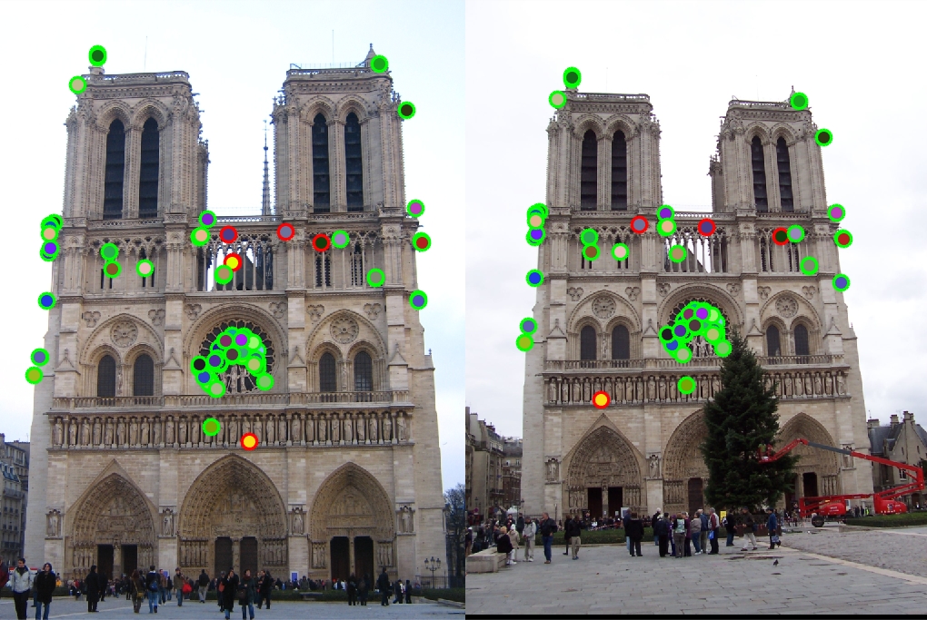
Results in a table

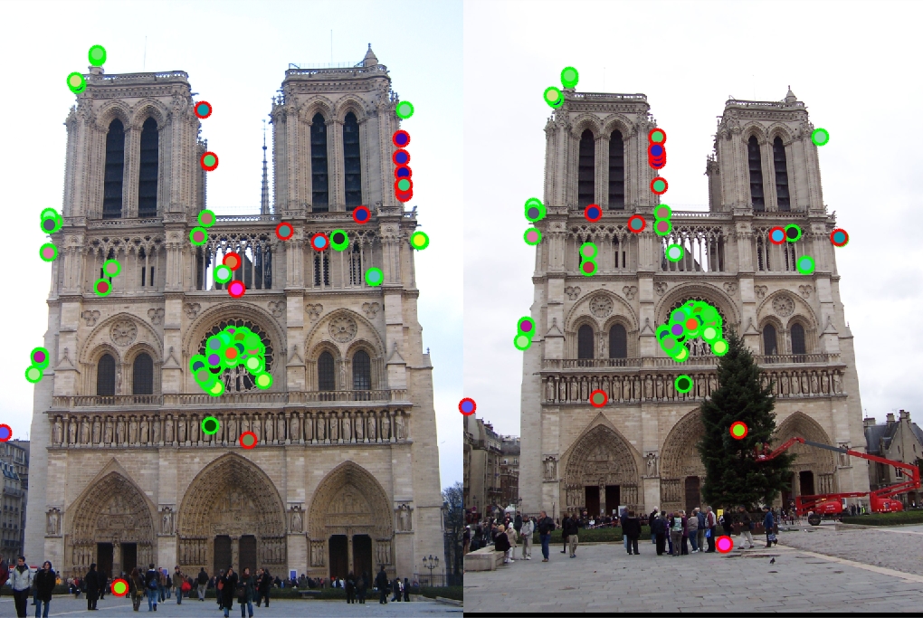
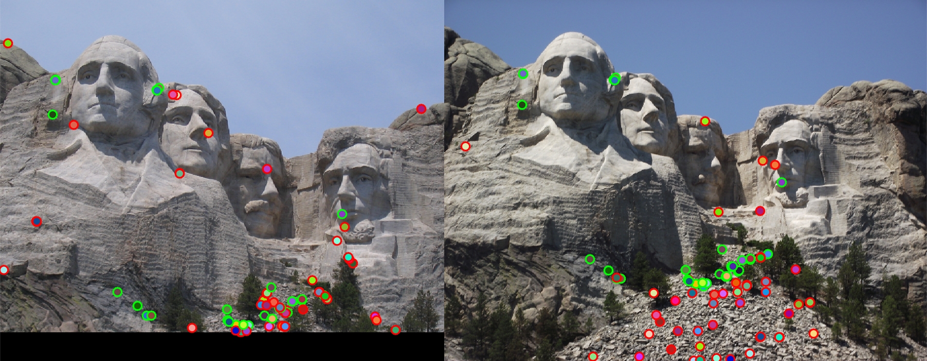
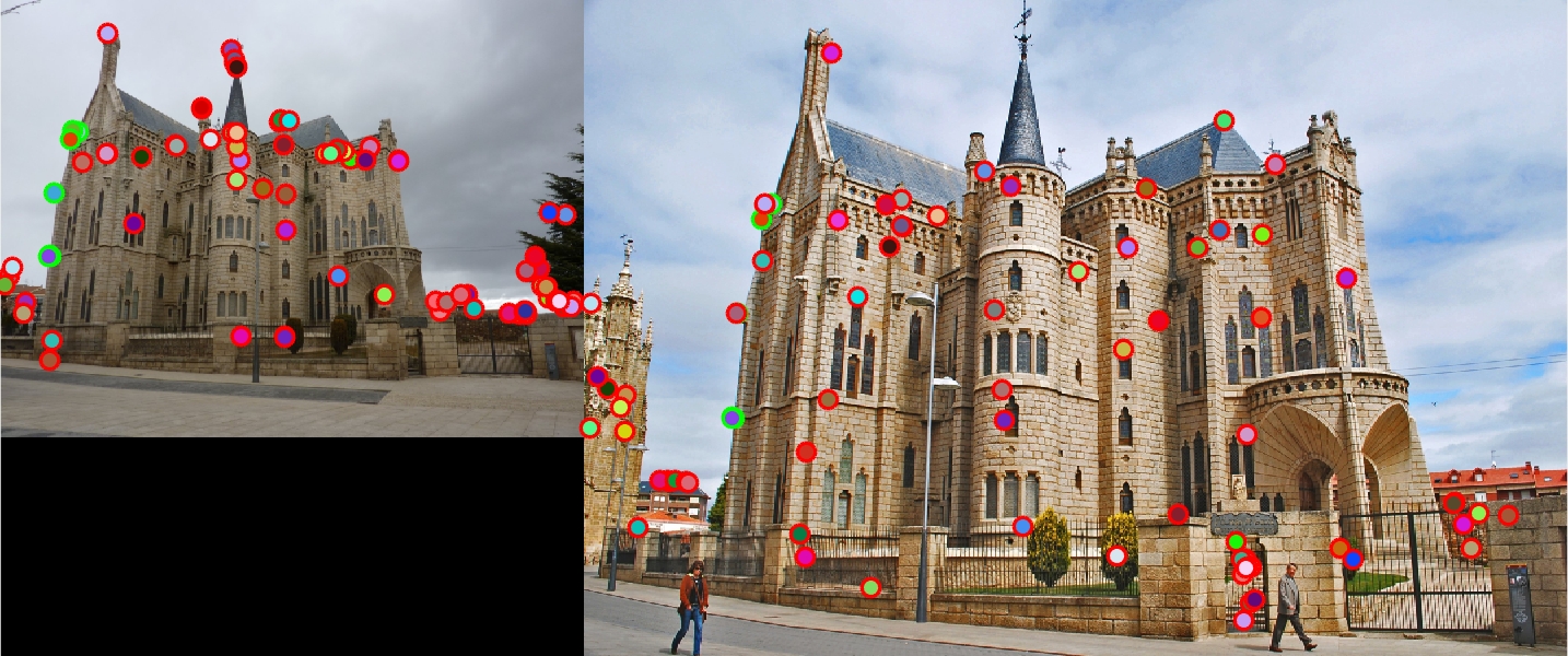
Left is original assignment, Right is gradient interpolation

Analysis

With the help of the small histogram improvement, for Notre Dame we get 93% correspondence for the top 100 pixels. For Mount Rushmore we get 39% correspondence while Episopal Gaudi gets only 8%. Notre Dame images had very similar orientation, scale, and color which aloud our algorithm to do well since we didn't implement orientation and scaling. Mount Rushmore images we're able to get a lot of matches at the top of the rock pile but had many mismatches for the points under the peak. This may be due to the first image being cropped and the second image having more interest points. Because many of the interest points were located around the rock pile, many of the hues and gradients may look very similar. The algorithm may have picked those interest points because the rocks created many corners. Episcopal Gaudi images were very hard for the algorithm because the scale and hues of the image were very different mainly the scaling was off. It was no surprise that since we didn't account for scaling of images, the interest points may have been totally missed on one image. I was implementing the scale extra credit, but for the sake of time I couldn't finish it. Overall when comparing two very similar images with very similar setups, the algorithm works ok. For the Notre Dame image, I was very excited that the algorithm matched the images around the center window.