Project 2: Local Feature Matching
Result of Matched Points
The goal of project 2 was to implement the Harris and SIFT interest point finding techniques in order to enable local feature matching. Scale invariance was not considered in this assignment. The tasks to be accomplished for this project can be divided as follows:
- I. Develop a Harris corner detector.
- II. Develop SIFT-like local feature describer.
- III. Match the corresponding features.
Harris Corner Detector
The Harris Corner Detector was devised by taking the gradient of the gaussian and convolving it to the image in the x and y directions respectively. Then, the equation for finding the R value was used to determine the corners of the image (R values above the threshold value, which in my case was 0.00005). Then, to find the local maximas of the interest points, the image was filtered with the maximum filter using the ordfilt2 function in MATLAB, and the pixel locations that are equal to the local maximum were chosen as corner locations.
Simplified Harris Detector code:
function [x, y] = get_interest_points(image, feature_width)
I = image;
g = fspecial('gaussian', round(feature_width/4), 1);
g2 = fspecial('gaussian', round(feature_width/8), 3);
[gx, gy] = imgradientxy(g);
Ix = imfilter(I,gx);
Iy = imfilter(I,gy);
gxx = imfilter(Ix.^2,g2)
gxy = imfilter(Ix.*Iy,g2);
gyy = imfilter(Iy.^2,g2);
alph = 0.06;
har = gxx.*gyy) - gxy.*gxy - alph * (gxx + gyy).^2;
di = ordfilt2(har,25,ones(5));
har = (har==di) & (har > 0.00005);
[y, x] = find(har);
Sift Feature Description
In order to apply a simplified version of SIFT, first, the derivatives of the gaussian were take in 8 directions. Then, those derivatives were convolved to the entire image. Note that the results of each convolution corresponds to the histogram in each directions. The next step was to take a 16x16 window around the interest point and to divide the window into 4x4 cells. In order to weigh the histogram from the distances of the pixels from the interest point, the gaussian of the 16x16 window was taken before dividing it into 4x4 cells. Then, the sum of the pixels in the window for the 8 orientations was taken. For each 16x16, the resulting feature descriptions were normalized by dividing each pixel by the magnitude of the window.
Feature Matching
Finally, features were matched by using the Nearest-Neighbor technique, where the ratios were taken by the distance from the interest point to the nearest point to the one that is the second closest. The confidence was evaluated by taking the reciprocal of the nearest neighbor distance ratio. For my case, the pdist2 function was used to find the Euclidean distance between the features of the first image and those of the next, and the resulting distances were sorted by closest to furthest. I also set a threshold value for the nearest-neighbor distance ratio to 0.75 such that ambiguous matches don't count.
Results
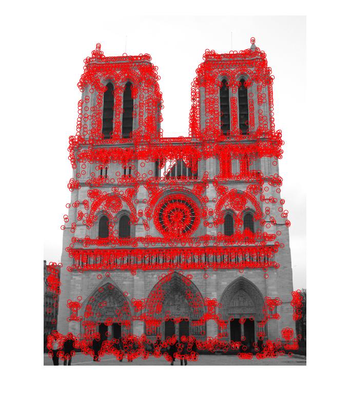
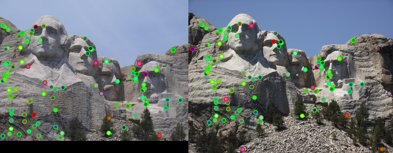
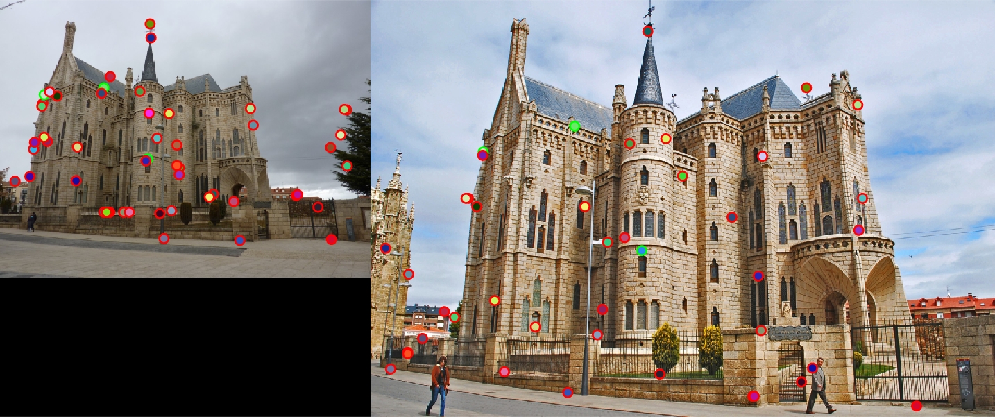
Corners detected by Harris corner detector 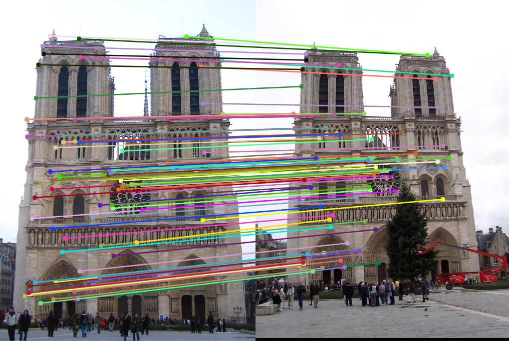
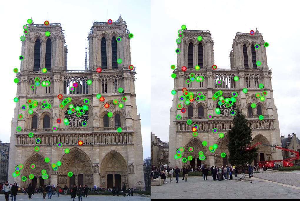
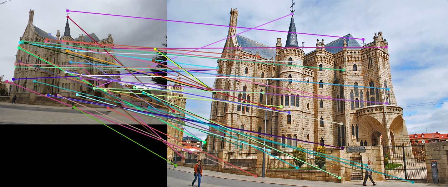
Matched features
Result of Matched Points |
The Notre Dame case showed 90% accuracy in feature matching.
|
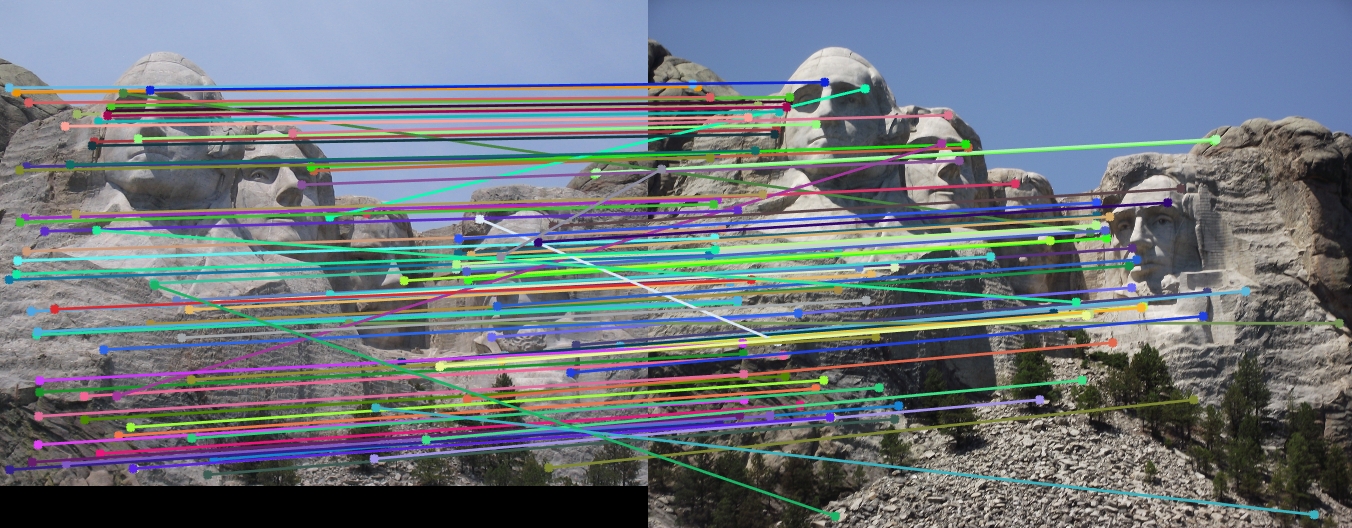
The Mount Rushmore case also showed 90% accuracy in feature matching.
|
The Episcopal Gaudi case unfortunately showed only 6% accuracy in feature matching.