James Mullenbach

Implementation details

For part 1, I split each image into windows and used the Harris corner detection algorithm to score each window based on its "cornerness". Then, I created a binary version of the original image by thresholding on the corner score. That is, if a window had corner score above the threshold, the center of the window became a 1 (white) in the resulting binary image. Then, as a method of non-maxima suppression, since many windows above the threshold could be grouped together, I found the maximum cornerness value from each connected white area of the binary image. The connected components were identified with MATLAB's bwconncomp() function. This method of non-maximum suppression both sped up the code and helped increase accuracy on the Notre Dame image set from 68% to 75%. The free parameters tweaked in this section were alpha, used in determining the Harris score, the threshold used in creating the binary image, and the size (width) of the square window. Tweaking these parameters helped by accuracy on the Notre Dame image set imcrease from 75% to 81%.

In part 2, I computed the histogram of gradients of various windows of the image, which would then be used as the constructed feature. This was done by first computing the horizontal and vertical edge-detected filtered versions of the image, created with the sobel filter. Then, at each window, the gradient was determined by taken the arctangent of the vertical and horizontal components. Finally, the angle was binned into one of 8 bins. Each window was separated into a grid of 4x4 sub-windows, each of which had its own 8-bin histogram, for a total feature of size 128. As suggested, I raised each histogram to a power slightly less than 1, which did improve accuracy. This exponent was then a free parameter. Initially, I implemented a simple feature comprised of just the (normalized) pixel values from each window. Moving from this simplistic feature to the histogram of gradients improved by accuracy on the Notre Dame image set from about 44% to 68%.

Finally, part 3 was implemented by simply computing the pair-wise distance between the 128-dimensional feature vectors in each image. Then, for each feature, the best match was defined as the one with the closest distance, with confidence defined using the nearest-neighbor ratio. Meaning, a feature whose closest feature is much closer than its second-closest feature will have high confidence. No free parameters were used in this section.

Example code

The MATLAB code below is a snippet from part 1 that builds the thresholded binary image based on the harris corner scores (with the score computation abstracted to a separate function).

window_width = 4;
[Gx, Gy] = imgradientxy(image);
dx = imgaussfilt(Gx);
dy = imgaussfilt(Gy);
alpha = 0.06;
threshold = 10;
bw = zeros(size(image));
% iterate over windows
for y_i = 1:size(image,1)-window_width+1
    for x_i = 1:size(image,2)-window_width+1
        %iterate within window to build matrix
        mat = getCornerness(dx, dy, x_i, y_i, window_width);
        harris = det(mat) - alpha * trace(mat).^2;
        if harris > threshold
            bw(y_i + floor(window_width/2), x_i + floor(window_width/2)) = 1;
        end
    end
end

Results in a table

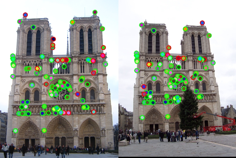
Full result for the Notre Dame image set - 81% accuracy. We can see strong correlations and matches between the features identified, with a few exceptions. One of the reasons this set was so successful was the similar vantage points, and the relative uniqueness of the ornate features on the building.

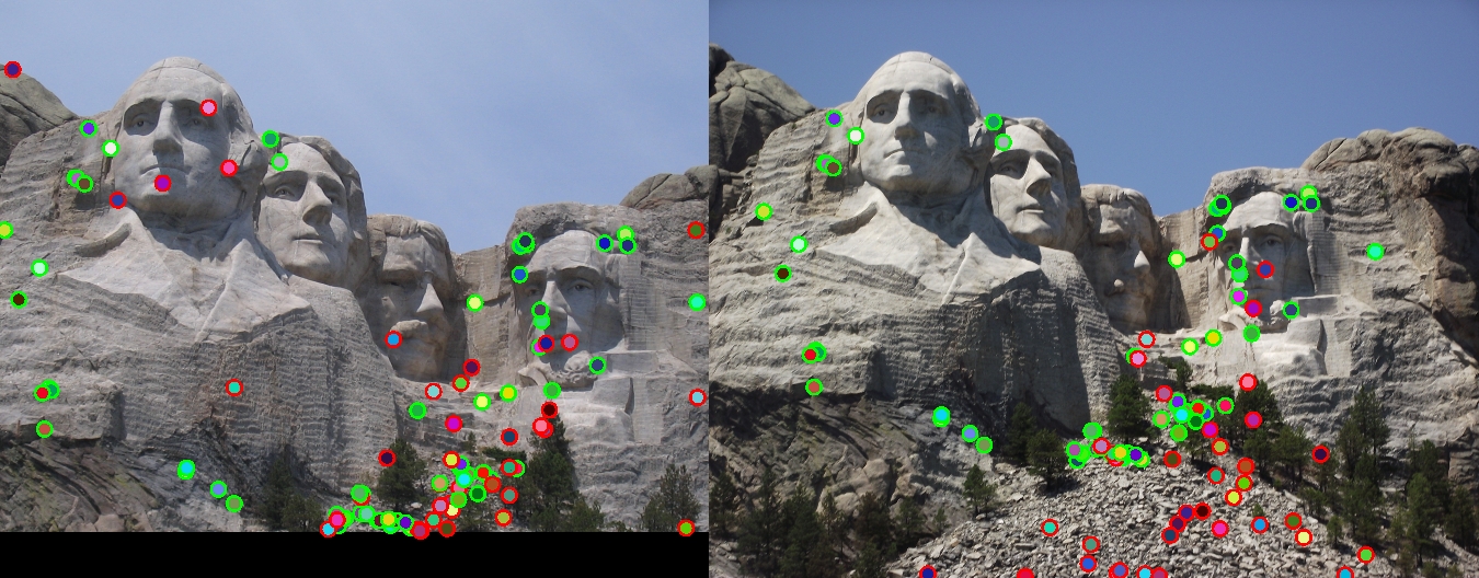
This set was more difficult, but I was able to achieve 61% accuracy on the top 100 feature matches. We see a lot of good matches, especially on the head of Lincoln, but the gravelly area below the monument (more prominent on the second image) leads to some discrepancy.

This image set was by far the hardest, and my algorithm performed by far the worst, at just 3% accuracy. One reason may be the very dissimilar distances at which the images were taken, but I suspect the most important difference is that the second image is much larger than the first. This could perhaps be mitigated by implementing something to improve the scale invariance in interest point detection (part 1). The lighting is also quite different.

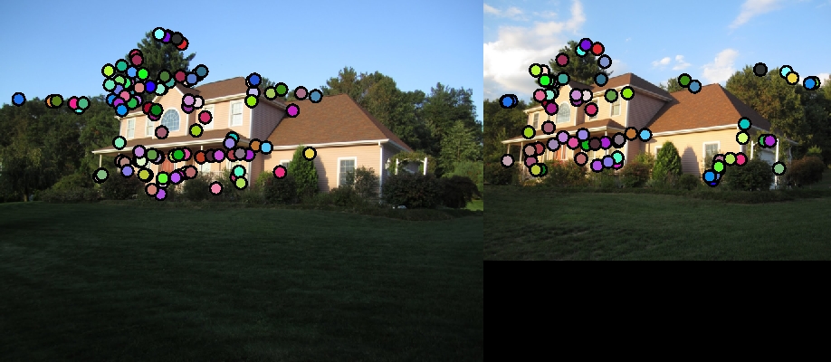
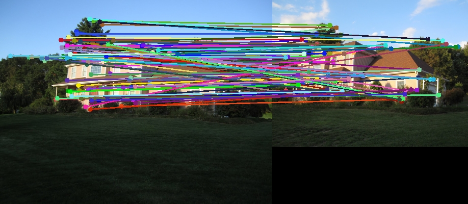
This example had no ground-truth correspondence, but we can see qualitatively that the matches are okay, somewhere between the Mt. Rushmore and Episcopal Gaudi examples. This image set I think also suffers from the lack of scale invariance, but we can still see that common sense matches occur, such as trees mapping to trees in other areas in the second image.

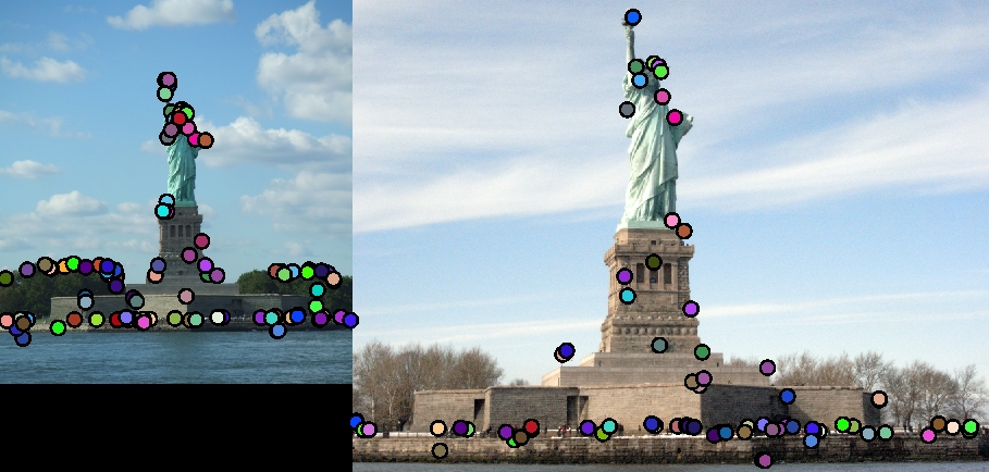
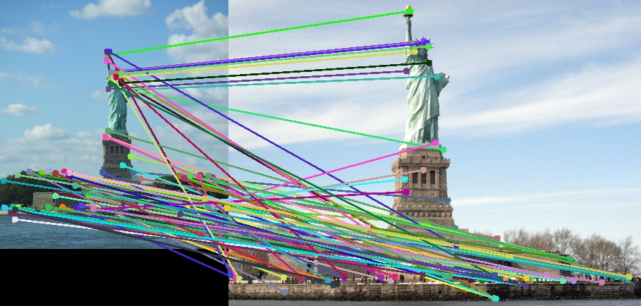
This is a second example without ground-truth correspondence. Again, the first thing I would do to fix the lack of correspondence here is implement scale invariance. We do see some good matches for the Statue of Liberty itself, however. The algorithm is much less accurate for other regions, though. One interesting observation is the trees do not match, as it is spring or summer in the first image and winter in the second image.