Project 2: Local Feature Matching
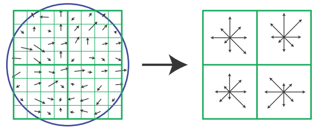
SIFT descriptor visualized. The left depicts image gradients, the right is the keypoint descriptor.
In this project, local feature matching was implemented with a 3-phase pipeline:
- Generate interest points from an image using Harris corner detection
- Use a SIFT-like descriptor to turn those interest points into quantifiable features
- Perform a matching algorithm based on the nearest neighbor ratio to identify matches
Detecting Interest Points
In order to detect the interest points on an image, I implemented the Harris corner detector as described in the textbook. This involves the following procedures:
- Construct a sobel filter for horizonal and vertical edges
- Convolve my image with the above filters to obtain derivatives in the x and y direction
- Use these values to reconstruct the Harris matrix as described in the textbook
- Compute the Harris cornerness value for pixels in the image via the evaluation formula
- Use a non-maxima suppression algorithm to highlight the most prominent interest points
Harris Corner Detection
The implementation for the evaluation function and non-maxima suppression can be seen below:
  %gradients
  sobelX = [1, 0, -1;
            2, 0, -2;
            1, 0, -1];
  sobelY = [1, 2, -1;
            0, 0, 0;
          -1, -2, -1];

  Ix = imfilter(image, sobelX);
  Iy = imfilter(image, sobelY);
  Ix2 = imfilter(Ix, sobelX);
  Iy2 = imfilter(Iy, sobelY);
  IxIy = imfilter(Ix, sobelX);

  %gausss
  gauss = fspecial('gaussian', 10, 1.0);
  Ix2 = imfilter(Ix2, gauss);
  Iy2 = imfilter(Iy2, gauss);
  Ixy = imfilter(IxIy, gauss);

  %corner detection quantified
  alpha = 0.06;
  det = (Ix2 .* Iy2) - Ixy .^ 2;
  trace = Ix2 + Iy2;
  interest = det - alpha .* (trace) .^ 2;

  %get rid of those boundaries
  %columns
  interest(1:feature_width, 1:size(interest, 2)) = 0;
  interest(size(interest, 1) - feature_width : size(interest, 1), 1:size(interest, 2)) = 0;
  %rows
  interest(1:size(interest, 1), 1 : feature_width) = 0;
  interest(1:size(interest, 1), size(interest, 2) - feature_width : size(interest, 2)) = 0;

  %threshold
  threshold = interest > 10*mean2(interest);
  interest = interest .* threshold;
  %sliding non-maxima suppression
  localMax = colfilt(interest, [feature_width feature_width], 'sliding', @max);
  interest = interest.*(interest == localMax);

  [y, x] = find(interest > 0);
Describing Features
The next phase of the pipeline is computing a descriptor for the interest points identified above. To accomplish this, I implemented a very basic version of the SIFT descriptor. Although seemingly simple, this approach was able to increase my accuracy to around 87% for the top 100 matches in the Notre Dame Model. This is an incredible step up from the ~40% accuracy I was obtaining via just the basic patching implementation. The procedure to create my descriptor can be summarized in the following steps:
- Create a 16x16 section around each interest point
- Break that section up further into a 4x4 grid
- Calculate the gradient angles from each 'cell' in the grid
- Obtain a histogram (of 8 possible orientations) for each cell
- Combine the histograms to obtain a 128-dimension SIFT descriptor for each interest point
- Perform cleanup such as normalization/square-rooting the features in an attempt to reduce the effect of contrast and gain
SIFT-like Descriptor
The gradient accumulation can be seen below:Square-rooting the features at the end was the only non-standard step performed, and it significantly increased accuracy.
        %find histograms at each cell
        currentGrid = zeros(1, 128);
        for d = 1 : size(dir, 1)
            currBins = zeros(1, 8);
            %Does the partitioning for me!!
            [~, ~, indices] = histcounts(dir(:, d), bins);
            %Note: indices holds the index of the bin each cell belongs to

            %accumulate gradient mags in bins
            for ind = 1 : length(indices)
                indexToAdd = indices(ind);
                currBins(indexToAdd) = currBins(indexToAdd) + mag(ind, d);
            end
            %add to correct position in grid
            currentGrid(1, 8*d - 7 : 8*d) = currBins;
        end
        %reduce contrast/gain by normalization
        currentGrid = currentGrid / norm(currentGrid);
        %add to return vector
        features(i,:) = currentGrid;
    end
    features = sqrt(features);
Matching Features
Once the descriptors have been created, all that's left to do is to match features between images. Unfortunately, I was only able to implement the naive approach to this matching problem: the ratio test. This test involves using Euclidian distances between features to find the ratio between the two closest neighobrs. If this ratio is less than a certain threshold value, it results in a match. This ratio test also returns a confidence level for matches, indicating the likelihood that a given pair is a 'good' match.
Nearest-Neighbor Ratio
My implementation of this test can be seen below:
  %threshold for confidence selection
  threshold = 0.80;

  %get distances between features and evaluate confidence ratio
  distances = pdist2(features1, features2, 'euclidean');
  [distances, f2] = sort(distances, 2);

  %  compute ratio
  allConf = distances(:,1)./distances(:,2);
  %filter on threshold
  filtered = allConf < threshold;
  %invert confidences
  confidences = 1 ./ allConf(filtered);

  %populate filtered matches
  matches = zeros(size(confidences,1), 2);
  matches(:,1) = find(filtered);
  matches(:,2) = f2(filtered, 1);

  % Sort the matches so that the most confident onces are at the top of the
  % list.
  [confidences, ind] = sort(confidences, 'descend');
  matches = matches(ind,:);
Results
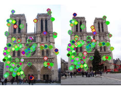
Top 100: 87 total good matches, 13 total bad matches. 87% accuracy |
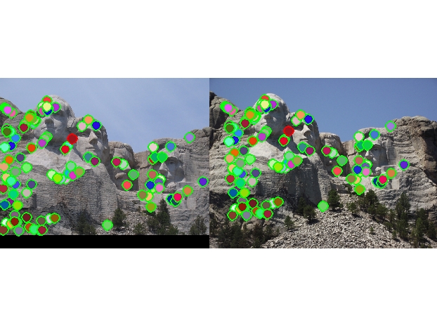
Top 100: 99 total good matches, 1 total bad matches. 99% accuracy |
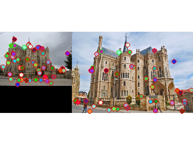
4 total good matches, 46 total bad matches. 8% accuracy |
No evaluation file provided, but evident that there is > 50% accuracy |
Overall, my implementation of the feature matching pipeline performed well. This can be observed in the high accuracy of the good to bad match ratio in the Notre Dame and Mt.Rushmore models. These images have distinct corners that are easy for my Harris detector to identify, and these images are of similar scale and orientation, meaning the SIFT descriptor can generate rather accurate features in the two images. To achieve these results, a lot of tinkering had to be done with some key parameters across the pipeline. The ones with the most impact on accuracy were the following:
- Threshold value used for identifying matches
- Sigma values for Gaussian filters used in the Harris corner detection algorithm
- The processing of the SIFT descriptor features vector after it was calculated (normalization, square-rooting)
- Using the top 100 confidence results instead of ALL matches